Corrosion Assessment of some Buried Metal Pipes using Neural Network Algorithm

Oparaodu et al., 2014 defined corrosion as the deterioration of metal or other materials brought about by

* Corresponding author. Tel.: +2348032351185

chemical, mechanical and biological action by soil environment. It may be caused by chemical reactions with carbonic acid, sulphuric acid or oxygen or by electrochemical metal ion transport. This definition of corrosion submits that by virtue of exposure of metals to the environment, corrosion is inevitable knowing fully well that exposed Iron materials and its popular alloy, Steel suffers the most. Emami, 2011 concludes that the annual cost of corrosion worldwide is over 3% of the world’s GDP. Even with this drawback, carbon steels have been on a wide application throughout the world. There are hundreds of thousands of kilometres of pipelines in various sectors of industry which include many uncoated pipelines in chemical manufacturing plants, interstate natural gas transmission lines, and offshore oil-and-gas production pipelines [Emami, 2011].

According to Oyewole, 2011, the high demand for oil and gas is still on the increase and pipes mostly made of carbon steel are recognized as the safest and most efficient way of transporting this product. With this fact, corrosion still remains a major problem in the transportation of oil and gas from where they are produced to where they are needed of which, pipelines buried beneath the earth are more prone to external degradation since the condition for corrosion to have effects on them are always present. These conditions are the presence of chemical substances such as Chloride, Oxygen (O 2 ), carbon dioxide (CO 2 ) hydrogen sulphide (H 2 S), water. Microbiological bacteria could also cause severe corrosion problems depending on the pH values, temperature, pressure, materials flow rate and flow profile of the system [Oyewole, 2011]. The consequences of this unwarranted natural phenomenon range from financial losses causing plant shut down, lost production, product loss, product contamination, fire accidents to loss of customer confidence and environmental degradation. Ekott et al., 2012 researched on external cathodic protection and control of the amount of H 2 S in the buried steel oil pipelines in Niger Delta to alleviate the effect of external corrosion but this was not able to effectively tackle the effect of external corrosion on these pipes, hence the need to revise this unworthy challenge.

To tackle this eminent set back, electroplating is widely employed to coat a metal with a thin layer of another metal. Of the various electrodepositing metals, nickel is one of the most often employed to increase the corrosion resistance or electrical conductivity of the underlying substrate [Sadiku-Agboola et al., 2012]. Some of the AISI 1015 steel pipe samples were Nickel plated, to be crossed assessed with the non-plated pipes of the same materials.

Of course, after preparing the electroplated specimens, there is usually a need to device a method to characterize the effectiveness of the electroplating. Most researchers nowadays find modelling as a useful tool to this end. Emami, 2011 describes one of the modelling tools as a means to solving real-world phenomena, investigate important questions about the observed world, explain real-world phenomena, test ideas and make predictions about the real world. The real world refers to; engineering, physics, physiology, ecology, wildlife management, chemistry, economics, sports and etc.

Having so many modelling tools to help interpret various daily activities, some tools have proven to be more versatile to the others. It is an incontestable fact that every human activity involves one mathematical problem or the other; the need to use mathematical modeling is increasing in modern times [Emami, 2011]. Matlab is a mathematical modeling and numerical computing environment which is undoubtedly one of the most widely used tools for drawing out relationships between far unrelated patterns of parameters. It allows easy matrix manipulation, plotting of functions and data, implementation of algorithms, creating user interfaces and interfacing with programs in other languages. The Neural Network Toolbox present in Matlab environment tools is used for designing, implementing, visualizing and simulating neural networks. It also provides comprehensive support for many proven network paradigms, as well as graphical user interfaces (GUIs) that enable the user to design and manage neural networks in a very simple way [].

Moreover, Artificial Neural Networks models have in general good performance even if one or more input parameters are unavailable. Lee and Kim, 2009 have been capable of expressing a variety of non-linear surfaces using a number of input-output training patterns that are selected from the entire design space in a global modified artificial neural networker. It gives us understanding into many real life processes and the interplay between or among variable(s) quantifying such models.

Sequel to this, Matlab with no doubt has placed at least a little confidence on researchers as per the viability of employing Artificial Neural Network models in executing these modelling related studies and has instilled a hope in this study for comprehensive modeling and analysis which is why it was principally used in this research work to carry out a comprehensive assessment..

Nomenclature
a, b, c, d	respective constants for each respective input
A	total surface area exposed
ANN	artificial neural network
CPR	corrosion penetration rate
D	density of the buried materials in (g)
I, J	number of input parameters considered together at once
K	number of output parameters
n	highest order of polynomial
sf	respective scaling factor for each input parameter considered
T	Time in (hrs)
W	respective weights for the inputs

2. Methods and Materials

A drawn out preliminary conclusion form the reviewed literatures submits that corrosion still remains one of the major drawback issues in the oil and gas industry. By reason of this, optimal characterization of corrosion resistant materials is of paramount essentiality.

The Methodology of this characterization therefore adopted the use of weight loss analysis for the determination of corrosion penetration rate. However, Modified Artificial Neural Network was afterwards used in clarifying the pattern of the corrosion effect together with the interpretation of the derived process algorithm for the analysis.

• 2.1.    Major Materials

The major materials used were:

• A.    AISI 1015 steel pipe

• a)    Nickel-plated

• b)    Non-electroplated

• B.    Soil samples: The soil samples were obtained from Pan-Ocean Corporation, Ovade Ogharefe, Delta state, Nigeria. It is an on-shore petroleum exploration and exploration site. 5 different soil samples were collected from 5 location points at the on-shore site. The locations were:

• a)    Tank farm

• b)    Skimmer pit

• c)    Export pump

• d)    Saver Pit

• e)    Arrival manifold point

• C.    Crude oil: This was gotten from the Shell Petroleum Development Company, North bank flow station, Obotobol, Forcados, Delta state, Nigeria.

• 2.2.    Experiment Procedure

Ten metal specimens were used. 5 were nickel electroplated specimens buried differently in the 5 different plastic containers containing soil samples while the other 5 non-plated specimens also buried into the same 5 soil samples but different plastic containers. In carrying out the experiment, the data were grouped into sets of input and output data. This is required so as to appropriately feed the modelling tool (Artificial Neural Network). The input data are:

• •    Temperature of the soil sample

• •    Temperature of the immediate surrounding

• •    pH of the soil sample

While the output data was:

• •    Weight loss

• 2.2.1.    Temperature of the soil samples

• 2.2.2.    Temperatures of the surroundings

• 2.2.3.    pH values of the soil samples

  From the reviewed literatures it was ascertained that the rate of corrosion is largely affected by the change in the pH values. This therefore made it highly required for it to be recorded from the experiment. Hanna brand pH metre of accuracy 0.1 was use, and the activity was carried out on site. On the first day, the pH meter was calibrated with a buffer solution of pH 4.0, then on the fourth day with a buffer solution of pH 10.0. This was necessary so as to allow for maximum accuracy of the pH metre. After taking all the pH readings, the soil minimum pH values for the non-electroplated and the electroplated specimens were 6.9 and 6.8 respectively while the maximum were 8.3 and 8.4. This conforms to the works of Oyewole, 2011.

This is the temperature of the soil samples having the steel specimens buried in them. The activity was carried out at the burial site with a laboratory thermometer of calibration -10 oC to 110 oC. This was to allow for actual temperature of the set-up affected by the corrosion as temperature change affects the rate of corrosion of a substance, as deduced from the literatures.

This is the temperature of the immediate surroundings of the whole set-up. For a better and more precise modelling, this parameter was recorded. Also, a laboratory thermometer of calibration -10 oC to 110 oC was used and it was carried out on-site.

The fig. 1 below shows the pH reading been collected at the soil sample 5 for the nickel-electroplated steel material with the digital pH meter.

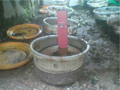
Fig.1. pH Reading for Nickel-Electroplated Soil Sample E

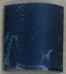
Fig.2. (a) Non-electroplated Steel Specimen; (b) Nickel-Electroplated Steel Specimen

• 3.    Result and Discussion

  • 3.1.    Analysis using Modified Artificial Neural Network

    Matlab R2009a was used extensively for generating expected results through compilation and execution of the codes. The reason for adopting this software is as a result of its capabilities and unmatched uses.

A function of Matlab is Artificial Neural Network (ANN). As postulated by Lee and Kim, 2009, ANN is one of the most efficient ways of solving complex problems bit by bit. Also, ANNs have the capacity to handle variety of non-linear surfaces using a number of input and output training patterns selected from the entire total field of possible data [Lee and Kim, 2009].

It was used in this study as a modelling tool on a series of seemingly unrelated input and output data collected to;

• a)    Train a pattern for the corrosion penetration rate

• b)    Investigate the effect of the input data in contribution to the corrosion penetration rate

• c)    Predict for outlying data accurately when computing in real life situations

• d)    Generate algorithms which could be used to propose for possible results of the output (corrosion

penetration rate) in the future when input data are varied

• e)    Plot graphs in various formats by manipulating data and executing simples codes

• 3.2.    Training of the Modified Artificial Neural Networks

• 3.3.    Encoding the Modified Artificial Neural Networks

The first task carried out on the modelling tool was training. Training in Artificial Neural Network is the process of exercising the modelling tool in order to allow it learns a particular pattern of behaviour before using it. The larger the number of data used for the training process, the more efficient and reliable the tool. This permits the tool to be able to handle a wide range of stochastic input data parameters efficiently. For this study, the whole 125 data collected for the 25 days was used to train the software.

As earlier stated, the network requires input and output data. The input data are the data recorded which contribute to the corrosion penetration rate of the buried specimens while the output data is the data recorded which results from the effect of the various input parameters. The input data recorded were:

• a.    Soil sample temperature

• b.    Immediate surrounding temperature

• c.    pH value

While the output data recorded was:

• a.    Weight loss

  The weight loss data recorded was afterwards translated to corrosion penetration rate. This was achieved by using the equation 1 below, as postulated by Emami, 2011:

87.6 x W D x A x T

CPR =

In computing the various CPR(s) for the corresponding weight loss values, Microsoft excel was used extensively. The results displayed on the Microsoft excel were imported to the Matlab environment for further modified artificial neural network analysis. This was due to the compatibility between the two computer software. The fig. 3 below shows the various input and output parameters for the neural network.

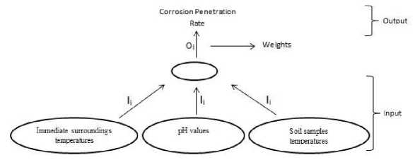
Fig.3. Input and Output Parameters for the Neural Network

Dealing with neural networks, there are various encoding formats but for this study, the codes were developed newly. Owing to this newly developed codes, the neural networks became modified thereby allowing for introduction of polynomial approximation (list square) format instead of the default neurons.

While modelling on the experiment on the modified artificial neural network, four cases where considered. The cases are:

• a.    All the three inputs

• b.    The first two inputs only

• c.    The first and the last inputs only

• d.    The last two inputs only

• 3.4.    Sequential overview of the algorithm

The fig. 4 below shows the flow chart for the modified artificial neural network.

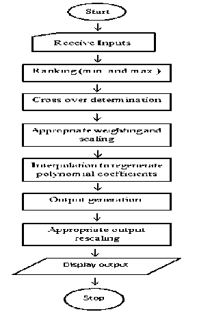
Fig.4. Flow chart for the Modified Artificial Neural Network

Following the flow chart on fig. 4 above, a sequential overview of the algorithm is however presented:

• a.    Start: This is a compilation initiation command.

• b.    Receive inputs: The input data received as been read from the Microsoft excel file saved in Matlab default folder are extracted into the Matlab memory.

• c.    Ranking: This is more of sorting out of the data. The first input which was the soil sample temperature was ranked. In respect of this, corresponding changes was applied across other input parameters which are immediate surroundings temperature and pH values, and the output parameter.

• d.    Cross-over determination: This is the estimation of the number of turning points present in the output (corrosion penetration rate). For this analysis, the turning points were constrained to 2. This gave rise to a cubic polynomial equation (i.e. order 3). In the data used there were more than 2 turning points with the changes in the values not critically high. From this, a line of best fit was drawn while approximating by

Table 1. Received Input and Output during Training

Baseline

Input	I 1	I 2	I 3	I 4
Input	J 1	J 2	J 3	J 4
Output	K 1	K 2	K 3	K 4

Table 2. Ranked Received Input and using Baseline

Ranked input	I 3	I 1	I 4	I 2
Ranked input	J 3	J 1	J 4	J 2
Ranked output	K 3	K 1	K 4	K 2

If

K >  к

K >  к 4

K 2 <  K 4

Then the number of cross overs could be determined from the ranked output.

Two cross over signifies that the data could be modelled using a polynomial of order 3 (i.e. a cubic equation). In modelling therefore, the following equations are used:

nn

£ Ki = a * n + b£ Ii + c£ Ii2(5)

i=1

nnn

£ KiI = a £ Ii + b £ Ii2 + c £ Ii3

i=1             i=1

nnn

£ Ki I2 = a £ Ii2 + b £ I3 + c £ Ii4

i=1               i=1

£ Ki = aI* n + bI £J + cI £,J?(8)

i=1

nnn

£ Ki J = aI £ J, + b £ J + cI £ J,3

i=1              i=1

nnn

£ Ki J2 = aI £ J^ + bI £ J,3 + cI £ J i=1                 i=1

• 3.4.1.    Case 1

The corrosion penetration rate is determined by all the three contributing factors, the soil temperatures, the immediate surroundings temperatures and the pH values. These factors are appropriately scaled and uniformly (unity) weighted. The validity of this case scenarios would be based on its deviation from the standard calculated CPR.

Number of input parameters considered = 3

n = 3

n

CPR = 0.33 * V ( a , + b, * x. + c. * x. ² + d. * x ,³ ) iiiii ii

i = 1

b = b * Sf * W.c. = c * Sf * W

d. = d * Sf * w

• 3.4.2.    Case 2

The corrosion penetration rate is determined by the first two contributing factors only, the soil temperatures and the immediate surroundings temperatures. These factors are appropriately scaled and uniformly (unity) weighted. The validity of this case scenarios would be based on its deviation from the standard calculated CPR.

Number of input parameters considered = 2

n = 3

CPR = 0.5 * У ( a, + b * x, + cx 2 + d * x, ³) i      i      i      ii        i      i

i = 1

bi = b * Sf * W

c = c * Sf * w

d = d * Sf * W i    ii

• 3.4.3.    Case 3

The corrosion penetration rate is determined by the first and the last contributing factors only, the soil temperatures and the pH values. These factors are appropriately scaled and uniformly (unity) weighted. The validity of this case scenarios would be based on its deviation from the standard calculated CPR.

Number of input parameters considered = 2

n = 3

CPR = 0.5 * У ( a ,. + b * x_f + cx 2 + d_f * x ³) i      i      i      ii        i      i

i = 1

b = b * Sf * wc. = c * Sf * Wd = d * Sf * w

• 3.4.4.    Case 4

The corrosion penetration rate is determined by the last two contributing factors, the immediate surroundings temperatures and the pH values. These factors are appropriately scaled and uniformly (unity) weighted. The validity of this case scenarios would be based on its deviation from the standard calculated CPR.

Number of input parameters considered = 2

n = 3

n

CPR = 0.5 * V (a. + b * x, + cx2 + d, * x3)

i      i      i      ii        i      i i=1

bi = b * Sfi * Wi

C = c * Sf * W dt = d * Sf * W

The scaling factors (Sf) are;

• • 0.1 for soil sample temperature

• • 0.1 for immediate surrounding temperature

• • 1 for pH value

• • 1000 for corrosion penetration rate

• 3.5.    Observation

• 3.6.    Graphical Representation of the Modified Artificial Neural Network Results

The numerical differences between the CPR values of the electroplated and the non-electroplated specimens are somewhat small.

Modified Artificial Neural Network was more extensively used for the analysis therefore, more interpretations were deduced from the generated graphical results. On each graph generated, there were five continuous lines having different colours. Each coloured line is interpreted as below:

• a)    Blue line: Plot for all the three input parameters as measured

• b)    Green line: Plot for all the three input parameters as modelled by the software

• c)    Red line Plot for the first two input parameters as modelled by the software

• d)    Cyan line: Plot for the first and the last input parameters as modelled by the software

• e)    Purple line: Plot for the last two input parameters as modelled by the software

The blue line which plots for the measured parameters serves as the reference for other plots. Other plots are modelled plots by the modified artificial neural networks.

The 2 graphs below in fig. 5 show the modified artificial neural network results for the electroplated and the non-electroplated specimens in sample 1. The plots for the four cases are distant from the measured (reference)

plot (blue line). This was due to a variation in training the tool.

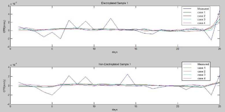
Fig.5. Modified Artificial Neural Network Graphical Result for Soil Sample 1 (Electroplated and Non-electroplated)

The 2 graphs below in fig.6 show the modified artificial neural network results for the electroplated and the non-electroplated specimens in sample 2. The plots for the four cases too are distant from the measured (reference) plot (blue line). This was also due to a variation in training the tool.

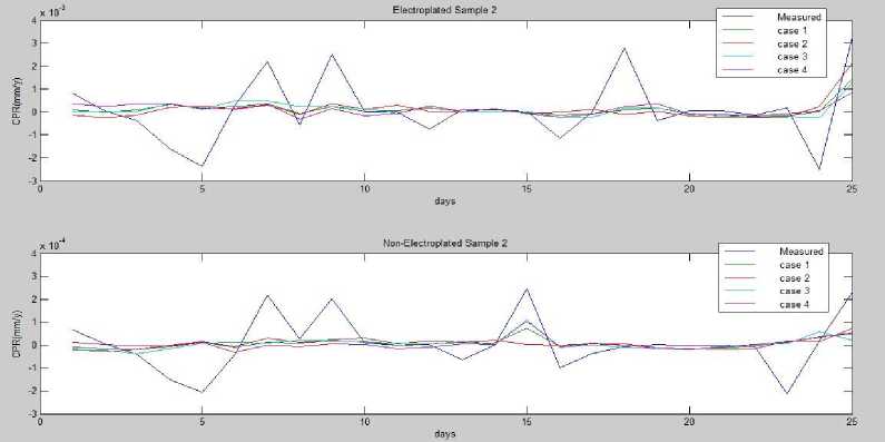
Fig.6. Modified Artificial Neural Network Graphical Result for Soil Sample 2 (Electroplated and Non-electroplated)

Here in fig. 7, the graphs show the modified artificial neural network results for the electroplated and the non-electroplated specimens in sample 3 to match well except for variations in days 13 and 15 in the case of the electroplated specimen and only day 17 in the case of the non-electroplated specimen. This was due to a variation in training the tool.

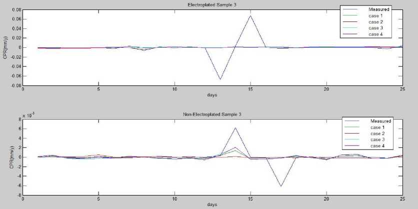
Fig.7. Modified Artificial Neural Network Graphical Result for Soil Sample 3 (Electroplated and Non-electroplated)

Unlike the earlier plotted graphs, the electroplated graph in fig. 8 below for the sample 4 matches so well that there were only two outlying data at days 1 and 2 whereas for the non-electroplated specimen, the graph did not really conform but conforms between days 9, 13, 19 23 and 25.

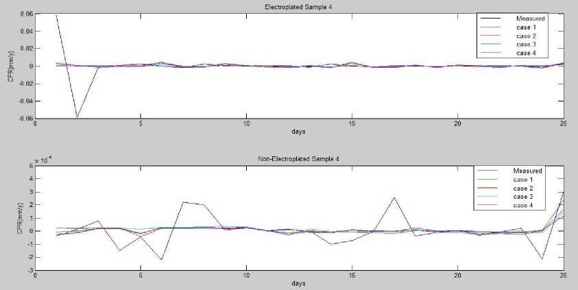
Fig.8. Modified Artificial Neural Network Graphical Result for Soil Sample 4 (Electroplated and Non-electroplated)

The results for specimens in sample 5 have two variations in their measured plots. For the electroplated specimen, the variations were at days 7 and 12 while for the non-electroplated specimen, the variations were at days 8 and 14.

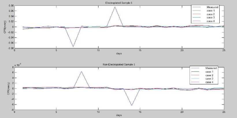
Fig.9. Modified Artificial Neural Network Graphical Result for Soil Sample 5 (Electroplated and Non-electroplated)

• 3.6.1.    Percentage errors

Determination of the relevance of each case was done by using the percentage error method on the modified artificial neutral network.

The results from the modified artificial neural network also include the percentage error for each case. This is presented below:

• •    Case 1: -4.0410e-013

• •    Case 2: -6.0080e-013

• •    Case 3: -4.3490e-013

• •    Case 4: -1.7660e-013

• 4.    Conclusions

  The key aim of this assessment which was to characterize the rate of corrosion of buried Nickel plated and non-plated AISI 1015 steel pipes using a Modified Artificial Neural Network on Matlab and taking the oil and gas area of Nigeria as a case study was successfully accomplished.

From the above results, the following was deduced; the cases listed below are arranged in an order of descending relevance to the corrosion penetration rate, i.e. case 2 had the strongest effect on the corrosion penetration rate while case 4 had the weakest effect on the corrosion penetration rate.

• •    Case 2: Soil sample temperature and the immediate surrounding temperature

• •    Case 3: Soil sample temperature and the pH

• •    Case 1: Soil sample temperature, immediate surrounding temperature and the pH value

• •    Case 4: Immediate surrounding temperature and the pH value

Clearly, both temperatures of the soil sample and the immediate surrounding when considered together have the greatest effect on the overall corrosion of the specimens, relative to the combined effects of the other parameters.

Also, Modified Artificial Neural Network relationships between the varied selected input parameters that affect the corrosion rate of some buried metal pipes (soil sample temperature, immediate surrounding temperature and pH value), and the output parameter (Corrosion Penetration Rate) were derived.

The major challenge that was faced during the course of this study was the non-availability of adequate funding to carry out extensively, the electroplating process by using several other coating metals that are equally competitive when it come to their ability to resist corrosion and also, the consideration of other parameters that enhances the corrosion of buried metal pipes like the actions of the soil microbacteria, presence of some chemical compound in the soil like the compounds of Sulphur, Nitrogen, Carbon etc, as seen in the reviewed literature. It is therefore proposed that these factors be considered in the subsequent studies for more robust results.

The authors are extremely grateful to the Department of Mechanical Engineering, University of Ibadan for providing space for our experimental test rig. Reviewers are equally appreciated for their valuable suggestions.

• [1]    Oparaodu KO, Okpokwasili GC. Comparison of percentage weight loss and corrosion rate trends in different metal coupons from two soil environments. International Journal of Environmental Bioremediation & Biodegradation. 2014; 2(5):243-249.

• [2]    Emami MRS. Mathematical modelling of corrosion phenomenon in pipelines.The journal of Mathematics and Computer Science. 2011;3(2):202-211.

• [3]    Oyewole A. Characterization of external induced corrosion degradation of Ajaokuta-Abuja gas pipeline system, nigeria. International Journal of Engineering and Technology. 2011;3(11):8061-8068.

• [4]    Ekott EJ, Akpabio EJ, Etukudo UI. Cathodic protection of buried steel oil pipelines in Niger Delta. Environmental Research Journal. 2012;6(4):304-307.

• [5]    Sadiku-Agboola O, Sadiku ER, Biotidara OF. The properties and the effect of operating parameters on nickel plating (review). International Journal of the Physical Sciences. 2012;7(3):349-360.

• [6]     http://www.mathworks.com/products/neuralnet

• [7]    Lee J, Kim T. A messy genetic algorithm and its application to an approximate optimization of an occupant safety system. Journal of Automobile Engineering. 2009;757-758.

• [8]    Kennedy JL. Oil and gas pipeline fundamentals. 2nd ed. PennWell Books; 1993.

• [9]    Malik AU, Andijani I. Corrosion Behaviour of Materials in RO water containing 250-350 PPM Chloride, International Desalination Association (IDA) World Congress Conference, Singapore. 2005; 1-13.

• [10]    Malik AU, Ahmad S, Andijani I, Al-Muaili F, Prakash, TL, O’Hara J. Corrosion Protection Evaluation of some Organic Coatings in Water Transmission Lines (Report No.TR 3804/APP 95009). Kingdom of Saudi Arabia: Saline Water Conversion Corporation. 1999.

• [11]    Samimi A. Causes of Increased Corrosion in Oil and Gas Pipelines in the Middle East. International Journal of Basic and Applied Sciences. 2013; 572-577.

• [12]    Yahaya N, Noor NM, Othman SR, Sing LK, Din MM. New Technique for Studying Soil-Corrosion of Underground Pipeline. Journal of Applied Sciences. 2011; 11(9):1510-1518.

• [13]    Monyei CG, Aiyelari T, Oluwatunde S. Neural Network Modeling of Electronic Waste Deposits in Nigeria: Subtle Prod for quick Intervention’ in proceedings of the iSTEAMS Research. Nexus Multidisciplinary Conference. 2013; 1(4):181-188.

• [14]    Abd El-Lateef MH, Abbasov VM, Aliyeva LI, Ismayilov TA. Corrosion Protection of Steel Pipelines Against CO2 Corrosion-A Review. Chemistry Journal. 2012; 2(2):52-63.

• [15]    Shen W. Developing a Reliable and Efficient Corrosion Resistance Characterization Technique for Magnesium Alloys Used in Automotive and Other Manufacturing Industries. Faculty Research Fellowship.

Bolaji Ahmed Oladipo (born September 6th, 1989) is a graduate of Mechanical Engineering from the University of Ibadan, Nigeria. Bolaji is a Computer Aided Design expert, programmer, instructor and research scholar who aspires to bag his PhD in Mechanical Engineering in the near future.

Olusegun Olufemi AJIDE (PhD) is a Lecturer 1 at the Department of Mechanical Engineering, University of Ibadan, Nigeria. He is a registered engineer (COREN) in Nigeria and a corporate member of Nigerian Society of Engineers. In addition, he is a registered corporate member, Nigerian Institution of Mechanical Engineers (NIMechE). His areas of research interests are materials development and characterization, Superalloys for aerospace applications, Fracture of structural materials, Failure analysis of engineering materials and applied dynamics/mechanics.

Chukwuka Monyei is currently a NRF-TWAS doctoral candidate at the Centre for Applied Artificial Intelligence, School of Mathematics, Statistics and Computer Science, University of KwaZulu Natal (UKZN). He is a masters graduate from the School of Electronic and Electrical Engineering at the University of Leeds and a first class graduate (BSc) from the Electrical and Electronic Engineering Department, University of Ibadan. Since 2014, he has been involved in research on the smart grid, energy management systems (EMS), demandside management (DSM) and distributed generation (DG) allocation/commitment scheduling and optimization.

e.

f.

g.

the lead square.

Appropriate weighting and scaling: Scaling was introduced so as to allow for convergence of all the data. This harmonises them to an approximately the same decimal fraction so they can relate well. This is appropriate because of the extreme nature of the values. Weighting on the other side tells the degree of contribution of an input over the other. But since the degree of contribution of the inputs had not been certified, they were all assumed to have the same relevance.

Interpolation to regenerate polynomial coefficient: This is the application of list square to establish a polynomial expression that generates a relationship between the CPR and all the inputs under consideration.

Output generation: The output computed.

• h.    Appropriate output rescaling: This recalled the scaling magnitude used earlier in step 5 and adjusted the output before displaying.

• i.    Stop: The computation ends.

The transitions obtained from the output matrix were thus used in generating the order of the polynomial function.

The first output was given as:

K (I) = al2 + bl + c

The second input was modelled similarly and used in generating the respective values of aI , bI and cI . The second output was thus given as:

K (J) = aIJ2 + bIJ + cI

The final output is therefore the average of the two equations 2 and 3:

K (I) + K (J) K =--------

2