Cosine-Based Clustering Algorithm Approach

Published Online February 2012 in MECS

In this paper, a new data clustering method is explored in the multidimensional spatial data mining problem. Spatial data mining is the discovery of interesting characteristics and patterns that may exist in large spatial databases. Usually the spatial relationships are implicit in nature. Because of the huge amounts of spatial data that may be obtained from satellite images, medical equipment, Geographic Information Systems (GIS), image database exploration etc., it is expensive and unrealistic for the users to examine spatial data in detail. Spatial data mining aims to automate the process of understanding spatial data by representing the data in a concise manner and reorganizing spatial databases to accommodate data semantics. It can be used in many applications such as seismology (grouping earthquakes clustered along seismic faults), mine- field detection (grouping mines in a minefield), and astronomy (grouping stars in galaxies) [1, 2]. The aim of data clustering method is to group the objects in spatial databases into meaningful sub- classes. Due to the huge amount of spatial data, an important challenge for clustering algorithms is to achieve good time efficiency. Also, due to the diverse nature of the spatial objects, the clusters may be of arbitrary shapes. They may be nested within one another, may have holes inside, or may possess concave shapes. A good clustering algorithm should be able to identify clusters irrespective of their shapes or relative positions. Another important issue is the handling of noise or outliers. Outliers refer to spatial objects which are not contained in any cluster and should be discarded during the mining process.

The results of a good clustering approach should not get affected by the different ordering of input data and should produce the same clusters. In other word, it should be ordered insensitive with respect to input data.

The complexity and enormous amount of spatial data may hinder the user from obtaining any knowledge about the number of clusters present. Thus, clustering algorithms should not assume to have the input of the number of clusters present in the spatial domain. To provide the user maximum effectiveness; clustering algorithms should classify spatial objects at different levels of accuracy. For example, in an image database, the user may pose queries like whether a particular image is of type agricultural or residential. Suppose the system identifies that the image is of agricultural category and the user may be just satisfied with this broad classification. Again the user may enquire about the actual type of the crop that the image shows. This needs clustering at hierarchical levels of coarseness which we call the multi-resolution property. In this paper, a spatial data mining method, termed Cosine Cluster is proposed. The multidimensional spatial data is considered as a multidimensional signal, and we apply signal processing techniques - Cosine transforms to convert the spatial data into the frequency domain. In Cosine transform, convolution with an appropriate kernel function results in a transformed space where the natural clusters in the data become more distinguishable, then the clusters are identified by finding the dense regions in the transformed domain. Cosine Cluster conforms to all the requirements of good clustering algorithms as discussed above. It can handle any large spatial data sets efficiently. It discovers clusters of any arbitrary shape and successfully handles outliers, and it is totally insensitive to the ordering of the input data. Also, because of the signal processing techniques applied, the multi-resolution property is attributed naturally to Cosine Cluster. To our knowledge, no method currently exists which exploits these properties of Cosine transform in the clustering problem in spatial data mining. It should be noted that the use of Cosine Cluster is not limited only to the spatial data, and it is applicable to any collection of attributes with ordered numerical values.

The rest of the paper is organized as follows. The related work is discussed in Section 2. In Section 3, the motivation behind using signal processing techniques for clustering large spatial databases is presented. This is followed by a brief introduction on cosine transform. Section 4 discusses our clustering method, Cosine Cluster and analyzes its complexity. In section 5, the experimental evaluation of the effectiveness and efficiency of Cosine Cluster using very large data sets is illustrated. Finally in Section 6, concluding remarks are offered.

• II.    Related Work

The clustering algorithms can be categorized into four main groups: partitioning algorithms, hierarchical algorithms, density based algorithms and grid based algorithms.

• A.    Partitioning Algorithms

• B.    Hierarchical Algorithms

Hierarchical algorithms create a hierarchical decomposition of the database. The hierarchical decomposition can be represented as a dendrogram. The algorithm iteratively splits the database into smaller subsets until some termination condition is satisfied. Hierarchical algorithms do not need K as an input parameter, which is an obvious advantage over partitioning algorithms. The disadvantage is that the termination condition has to be specified. BIRCH (Balanced Iterative Reducing and Clustering using Hierarchies) [21] uses a hierarchical data structure called

CF-tree for incrementally and dynamically clustering the incoming data points. CF-tree is a height balanced tree which stores the clustering features. BIRCH tries to produce the best clusters with the available resources. They consider that the amount of available memory is limited (typically much smaller than the data set size) and want to minimize the time required for I/O. In BIRCH, a single scan of the dataset yields a good clustering, and one or more additional passes can (optionally) be used to improve the quality further. So, the computational complexity of BIRCH is O(N). BIRCH is also the first clustering algorithm to handle noise [21]. Since each node in CF-tree can only hold a limited number of entries due to its size, it does not always correspond to a natural cluster [21]. Moreover, for different orders of the same input data, it may generate different clusters. In other word, it is order-sensitive. Also as our experimental results show, if the clusters are not “spherical” in shape, BIRCH does not perform well. This is because it uses the notion of radius or diameter to control the boundary of a cluster.

• C.    Density Based Algorithms

Pauwels et al proposed an unsupervized clustering algorithm to locate clusters by constructing a density function that reflects the spatial distribution of the data points [4]. They modified non-parametric density estimation problem in two ways. Firstly, they use crossvalidation to select the appropriate width of convolution kernel. Secondly, they use Difference-of-Gaussians (DOG's) that allows for better clustering and frees the need to choose an arbitrary cut off threshold. Their method can find arbitrary shape clusters and does not make any assumptions about the underlying data distribution. They have successfully applied the algorithm to color segmentation problems. This method is computationally very expensive [4]. So it can make the method impractical for very large databases. Ester et al presented a clustering algorithm DB- SCAN relying on a density-based notion of clusters. It is designed to discover clusters of arbitrary shapes [3]. The key idea in DBSCAN is that for each point of a cluster, the neighborhood of a given radius has to contain at least a minimum number of points, i.e. the density in the neighborhood has to exceed some threshold. DBSCAN can separate the noise (outliers) and discover clusters of arbitrary shape. It uses R*-tree to achieve better performance. But the average run time complexity of DBSCAN is O(NlogN).

• D.    Grid-Based Algorithms

Recently a number of algorithms have been presented which quantize the space into a finite number of cells and then do all operations on the quantized space. The main characteristic of these approaches is their fast processing time which is typically independent of the number of data objects. They depend only on the number of cells in each dimension in the quantized space. Wang et al proposed a STatistical INformation Grid-based method (STING) for spatial data mining [20]. They divide the spatial area into rectangular cells using a hierarchical structure. They store the statistical parameters (such as mean, variance, minimum, maximum, and type of distribution) of each numerical feature of the objects within cells. STING goes through the data set once to compute the statistical parameters of the cells, hence the time complexity of generating clusters is O(N). The other previously mentioned clustering approaches do not explain if (or how) the clustering information is used to search for queries, or how a new object is assigned to the clusters. In STING, the hierarchical representation of grid cells is used to process such cases. After generating the hierarchical structure, the response time for a query would be O(K), where K is the number of grid cells at the lowest level [20]. Usually K << N, which makes this method fast. However, in their hierarchy, they do not consider the spatial relationship between the children and their neighboring cells to construct the parent cell. This might be the reason for the isothetic shape of resulting clusters, that is, all the cluster boundaries are either horizontal or vertical, and no diagonal boundary is detected. It lowers the quality and accuracy of clusters, despite the fast processing time of this approach.

Wave Cluster, which is a grid-based approach is very efficient, especially for very large databases. The computational complexity of generating clusters in our method is O(N). The results are not affected by outliers and the method is not sensitive to the order of the number of input objects to be processed. Wave Cluster is well capable of finding arbitrary shape clusters with complex structures such as concave or nested clusters at different scales, and does not assume any specific shape for the clusters. A priori knowledge about the exact number of clusters is not required in Wave Cluster. However, an estimation of expected number of clusters, helps in choosing the appropriate resolution of clusters, we proposed Cosine Cluster, which is a grid-based approach too, but it is different from Wave Cluster by the way of transformation in Cosine Cluster. We used cosine transformation instead of wavelet transformation for more efficiency discarding outliers (noise), and it has the same features of the Wave Cluster with slightly difference in performance. [22]

• III.    Cosine-Based Clustering

• A.    Discrete Cosine Transform

Discrete cosine transform (DCT) has become the most popular technique for image compression over the past several years. One of the major reasons for its popularity is its selection as the standard for JPEG. DCTs are most commonly used for non-analytical applications such as image processing and signal processing DSP applications such as video conferencing, fax systems, video disks, and HDTV. DCTs can be used on a matrix of practically any dimension. Mapping an image space into a frequency space is the most common use of DCTs. For example, video is usually processed for compression/ decompression as 8 x 8 blocks of pixels. Large and small features in a video picture are represented by low and high frequencies. An advantage of the DCT process is that image features do not normally change quickly, so many DCT coefficients are either zero or very small and require less data during compression algorithms. DCTs are fast and like Fast Fourier Transforms (FFTs), require calculation of coefficients. The entire standards employ block based DCT coding to give a higher compression ratio. Various different techniques and algorithms employed for DCT. The basic difference between DCT and wavelets is that in wavelets rather than creating 8 X 8 blocks to compress, wavelets decompose the original signal into sub-bands. Wavelets are basically an optimizing algorithm for representing a lot of change in the pictures. With DCT algorithm, the 8 X 8 blocks can lose their crisp edges, whereas, with wavelets the edges are very well defined. We will not go in detail with the differences between wavelets and DCT but we just want to mention it to prove our case for the proposal of DCT for multi-resolution analysis. There is another compression method being developed call Fractals which is based on quadratic equations. This method is very well suitable with images which have patterns or a lot of repetitions.

Now, if the wavelets produce much better results than DCT then why do we need to try DCT for multiresolution? The reason is that there are certain drawbacks to wavelets especially in terms of computation time required, as for the highest compression rates it takes a longer time to encode [23].

• B.    Multi-Resolution Analysis

  The concept of multi-resolution analysis was formally introduced by Mallat [1989] and Meyer [1993].Multi-resolution analysis provides a hierarchical structure. It means that in order to get 15 % compression, the image is not compressed directly to 15% as in block DCT, instead the image is compressed in stages; reducing the image to a half at every stage. At different resolutions the details of a signal generally characterize different physical aspects of the image or a signal per say. It is a common observation that at coarse resolutions the details correspond to larger overall aspects of the image while at fine resolutions the distinguishing features are prominent. Some of the common applications of multi-resolution analysis are image compression, edge detection, and texture analysis. Multi-resolution analysis is not only restricted to the previously mentioned techniques but recently researchers also found some more applications of multi-resolution analysis and found good results. These applications include image restoration and noise removal. Multi-resolution analysis tries to understand the content of the image at different resolutions. Wavelet analysis makes use of the notion of multi-resolution analysis. Wavelet analysis is built on Fourier analysis and it was designed to overcome the drawbacks of the Fourier analysis. According to Meyer [1992], the most powerful tool for the construction wavelets and for the implementation of the wavelet decomposition and reconstruction algorithms is the notion of multi-resolution analysis. The concept of multi-resolution analysis was formally introduced by Mallat [1989] and Meyer [1993].

Multi-resolution analysis provides a convenient framework for developing the analysis and synthesis filters. The basic components for a multi-resolution analysis are: an infinite chain of nested linear function spaces and an inner product defined on any pair of functions. Multi-resolution has been widely used recently with great success with the wavelets. Wavelets and multiresolution analysis have received immense attention in the recent years. There have been a lot of problems which have made use of wavelets and multi-resolution analysis and thus making it a popular scheme for compression. The basic idea behind multi-resolution analysis is to decompose a complicated function into smaller and simpler low resolution part together with wavelet coefficients. These coefficients are very important to recover the original signal when we apply the inverse. Mallat [1989] described multi-resolution representation as a very effective method for analyzing the information content for images. Mallat and Meyer were the pioneers in the theory of multi-resolution analysis. For this reason, most of this section is written under the influence of the paper written by Mallat in 1989. The original scale and size of objects in an image depends upon the distance between the image and the camera. To compress an image to a smaller size, we ought to keep the essential information of the image. In Mallat’s words, a multiresolution decomposition enables us to have a scaleinvariant interpretation of the data.

• C.    Cosine Vs Wavelet Transform

As mentioned in the introduction section, researches have been erroneous in comparing JPEG with wavelets as a means of comparing DCT and wavelets. Discrete cosine transforms and wavelets have been popular techniques used in signal processing for quite some time. Many researches have been comparing these two techniques to decide which one is superior. The results of such comparisons have suggested that wavelets outperform DCT by a big margin. This is not a fair comparison due to the fact that JPEGs only use a part of the discrete cosine transform. Discrete cosine transform is far more powerful and performance efficient than what JPEG can offer. JPEG uses 8 X 8 blocks which are then transformed into 64 DCT coefficients. This is a very low number because when we do the compression we make the coefficients 0s and in this case we are not left with much of the information when we convert some of the coefficients out of 64 to 0s. We can have far better results if we use larger block sizes such as 32 x 32. It will only be fair to run a performance comparison between wavelets and discrete cosine transform because the hardware implementation of discrete cosine transform is very less expensive than wavelets and it is well acknowledged. The other important consideration while comparing wavelets and Discrete cosine transform is to keep the quantizer same. Various quantization schemes are available to be used with different transforms. Far better results can be obtained from discrete cosine transform than the standard JPEG if the new improved methods are employed. These methods include Q-matrix design, optimal threshold and joint optimizations. The results from the experiments indicate that a gain of 1.7 dB was achieved with joint optimization over the standard JPEG with the same bit rate. The standard JPEG is, in fact, not optimal and even JPEG with its limited DCT use can still be improved. In order to stay compatible with JPEG in DCT based embedded image coding is compared with wavelet based JPEG like image coding. In wavelet –o0'based JPEG like image coding, the DCT in baseline JPEG is replaced by a three level wavelet transform. This way the performance of the wavelet transform is achieved while staying compatible with JPEG. Image coding mainly depends on what kind of entropy coder and quantizer used rather than the difference between the wavelets and DCT. This observation is a benchmark in the comparison of DCT and wavelets. There is actually not a big difference between DCT and wavelets but in fact the difference lies in choice of quantizer and entropy coder. For still images, the difference between the wavelet transform and the discrete cosine transform is less than 1 dB and for video coding this difference tends to be even smaller. This results obtained are very important because of the fact that JPEG and discrete cosine transform are erroneously used interchangeably in research and in comparing wavelets with DCT. DCTs can do much more and much better than what the baseline JPEG can offer. One of the major critiques of the standard DCT is the blocking effect that becomes more prominent at higher compression ratios. This blocking effect and other properties of DCT will be explored in detail in the next chapter. As already mentioned, the standard JPEG is based on DCT while an 11 improved version of JPEG, known as JPEG2000, is based on wavelets and it is supposed to solve the problem of blocking artifacts in standard DCT. There are quite many benefits of JPEG2000 over the standard JPEG. JPGE2000 makes use of the multi-resolution analysis and that’s why it is pertinent to mention JPEG2000 here, and in comparison with the standard JPEG which use the standard 8x8 block DCT. The main features of JPEG2000 are: its superior low bit rate performance which enables it to attain higher compression without the loss of the information data, its multiple resolution representation, lossy and lossless compression, and region of interest (ROI) coding etc. Below some examples for compressed images are shown at different bits per pixel to illustrate the difference between the 8x8 block DCT and wavelets based JPEG2000. It is very clear in these images that the blocking effect becomes more prominent at higher compressions and lower bit rates.

(a)

only be considered as the comparison between 8x8 block DCT and wavelets because there are several different new techniques that improve DCT considerably.

• D.    DCT Formal Definition

As mentioned earlier, the DCT transform de-correlates the image data. In DCT, an image is typically broken into 8x8 blocks. These blocks are each transformed into 64 DCT coefficients. The most commonly used DCT definition of one dimensional sequence of length N is

(b)

Figure 3.1: (a) block DCT at 12.5%; (b) JPEG 2000 at 12.5%

С(и) = « (и) I ";! f(x)cos [ "(²f"^1u ]               (3.3)

(a)

The above equation is defined for u = 0, 1, 2, 3…..N-1. There are two kinds of DCT coefficients; AC and DC. The DC coefficient corresponds to the value of C (u) when u = 0. In other words, DC coefficient provides the average value of the sample data. The rest of the coefficients are called AC coefficients. Based on the one dimensional DCT as described above, the two dimensional DCT can be achieved.

C⁽U,V) = «(и)« (v) Y ";^{1 Z} y=oV (f, y)cos [ "(Zf^ cos^ ²^¹)" ] (3.4)

The above equation shows the two dimensional DCT. It is clear from the above equation that it is derived by multiplying the horizontal one dimensional basis function with the vertical one dimensional basis function. Both one and two dimensional DCTs work in similar fashion. One dimensional DCT is used mainly in sound signals because of its one dimensional nature, whereas, two dimensional DCT is used in images because of their two dimensional nature.

(b)

Figure 3.2: (a) block DCT at 25 %; (b) JPEG 2000 at 25%

Figures 3.1 and 3.2 clearly demonstrate the difference between the wavelets and the block DCT. It is also clear from the above images that higher the compression ratio, the more the blocking effects in the image. This should

• IV.   Proposed algorithm

A． Multi-model algorithm introduction

Given a set of spatial objects O i , 1 <  i <  N , the goal of the algorithm is to detect clusters and assign labels to the objects based on the cluster that they belong to. The main idea in Cosine Cluster is to transform the original feature space by applying cosine transform and then find the dense regions in the new space. It yields sets of clusters at different resolutions and scales, which can be chosen based on users' needs. The main steps of Cosine Cluster are shown in Algorithm 1.

Algorithm 1

Input: Multidimensional data objects’ feature vectors

Output: clustered objects

• 1.    Quantize feature space, then assign objects to the units.

• 2.    Apply cosine transform on the feature space.

• 3.    Find the connected components (clusters) in the transformed feature space, at different levels.

• 4.    Assign label to the units.

• 5.    Make the lookup table.

• 6.    Map the objects to the cluster

• B.    Step 1: Quantization

Each i dimensional of the d-dimensional feature space will be divided into m_i intervals; this process is called quantization (Quantize Feature Space), which is the first step of Cosine Cluster algorithm. If we assume that m i is equal to m for all the dimensions, there would be m^d units in the feature space. Then the objects will be assigned to these units based on their feature values. Let F k = ( f 1 , f 2 , . . . , f d ) be the feature vector of the object o k in the original feature space. Let M j = ( v 1 , v 2 , . . . , v d ) denote a unit in the original feature space where v i , 1 ≤ v i ≤ m i , 1 ≤ i ≤ d , is the location of the unit on the axis X i of the feature space. Let s_i be the size of each unit in the axis X_i . An object ok with the feature vector F k = ( f 1 , f 2 , . . . , f d ) will be assigned to the unit M_j = ( v₁ , v₂ , . . . , v_d ) if

Vi ⁽ v - 1)s ; <  f_t <  v_ts_b    1 < i < d

The number (or size) of these units is an important issue that affects the performance of clustering.

• C.    Step 2: Transform

The second step in Cosine Cluster algorithm is applying discrete cosine transform on the quantized feature space. Discrete cosine transform will be applied on the units Mj results in a new feature space and so new units Tk. Cosine Cluster detects the connected components in the transformed feature space. Each connected component is a cluster which is a set of units Tk. For each resolution r of cosine transform, there is a set of clusters CT, but usually number of clusters is less at the coarser resolutions. In our experiments, cosine transform was applied three times and we tried Haar, Daubechies, Cohen-Daubechies-Feauveau ((4,2) and (2,2)) transforms [19, 7, 18, 22]. Average sub bands (feature spaces) approximate the original feature space at different scales, which help in finding clusters at different level of details. We use the algorithm in [12] to find the connected components in the 2-dimensional feature space (image).The same concept can be generalized for higher dimensions.

• D.    Step 4: Label and Make Look Up Table In the fourth step of the algorithm, Cosine Cluster labels the feature space units which are included in a cluster, with its cluster number. That is,

Vc VT_k,T_k ec ^ l_Tk= c „ c e C_r, where l_Tk is the label of the unit T_k . The clusters which are found cannot be used directly to define the clusters in the original feature space, since they exist in the transformed feature space and are based on wavelet coefficients. Making a lookup table LT is made by the Cosine cluster to map the transformed feature space units to the units in the original feature space. Cosine Cluster makes a lookup table LT to map the units in the transformed feature space to the units in the original feature space. Each entry in the table specifies the relationship between one unit in the transformed feature space and the corresponding unit(s) of the original feature space. So the label of each unit in the original feature space can be easilydetermined. Finally, Cosine Cluster assigns the label of each unit in the feature space to all the objects whose feature vector is in that unit, and thus the clusters are determined. Formally,

Vc VM j , Vo_; e M j , l₀. = c_n,c e C_T,    1

Where l₀ . is the cluster label of object o_; .

• V.   Performance Evaluation

In this section, we evaluate the performance of Cosine Cluster and demonstrate its effectiveness on different types of distributions of data. Tests were done on synthetic datasets generated by us and also on datasets used to evaluate BIRCH [21]. We mainly compare our clustering results with BIRCH. We first introduce the test datasets.

• A.    Synthetic Datasets

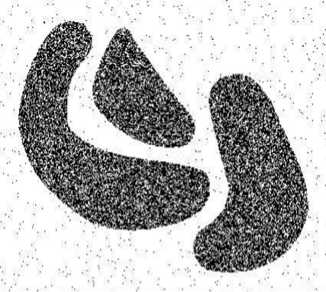
  Datasets DS1, DS2 and DS3 are the same as used by [21]. They are shown in Figure 6 a, b, and c. Each dataset consists of 100,000 points. The points in DS3 are randomly distributed while DS1 and DS2 are distributed in a grid and sine curve pattern respectively. The other datasets shown in Figure 6 were generated using our own dataset generator. Data set DS4 is the noisy version of DS5 that is generated by scattering 1000 random noise points on the original dataset.

• B.    Clustering Huge Datasets

All the datasets used in the experiments contain typically more than 10,000 data points. DS1, DS2 and DS3 each one has 100,000 data points. Cosine Cluster can successfully handle arbitrarily large number of data points. Figure 5.1 shows Cosine Cluster’s performance on DS1. This map coloring algorithm has been used to color the clusters. Neighboring clusters have different colors. But non-neighboring clusters might be allocated the same color.

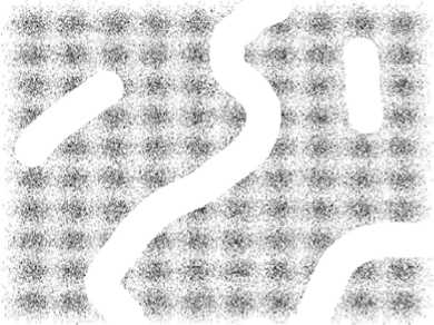
Figure 5.1: Cosine Cluster in DS1

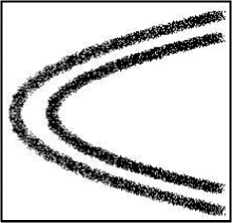
• C.    Clustering Arbitrary Shapes

As we mentioned earlier, spatial data mining methods should be capable of handling any arbitrary shaped clusters. There are 3 arbitrary shaped clusters in dataset DS5. Figure 5.3-a shows Cosine clustering of DS5. Figure 5.3-b shows BIRCH clustering for the same data set. This result emphasizes deficiency of the methods which assume the shape of the clusters a priori.

ж-^- r<1H*w w

Hwfr***- ^ ^ # ^ < ^*^ w ^ -

^■'M ^^;^.^S ^ '^ ^M

• #• ^ e- .^- -^ ^ < ^ ^ ■^•

• a) DS1

  

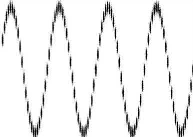
  b) DS2

  
  
  

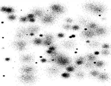
  c) DS3

  
  
  

  d) DS4

  
  
  

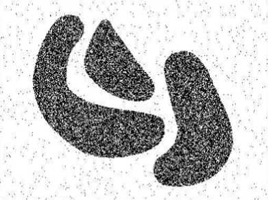
  e) DS5

  
  
  

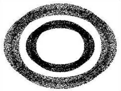
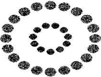
  f) DS6

  
  
  

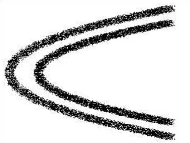
  g) DS7

  
  
  

  h) DS8

  
  

Figure 5.2: The datasets used in the experiments.

a)

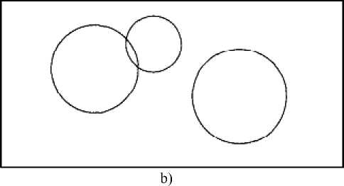
Figure 5.3: a) Cosine Cluster on DS5; b) BIRCH on DS5

a)    Handling Outliers

This result emphasizes deficiency of the methods which assume the shape of the clusters a priori. Cosine Cluster is very effective in handling outliers. Figure 5.4 shows clustering achieved by Cosine Cluster on DS4 dataset (noisy version of DS5 dataset). It successfully removes all random noise and produces three intended clusters. Also, because of O(K) (where K is the number of grid points), the time complexity of the processing phase of Cosine Cluster , that is, the time taken to find the clusters in the noisy version of the data is the same as that on without noise.

Figure 5.4: Cosine Cluster on DS4.

• b)    Clustering Nested and Concave Patterns Cosine Cluster can successfully cluster any complex pattern consisting of nested or concave clusters. From Figure 6-f and Figure 5.5-a, we see that Cosine Cluster’s result is very accurate on nested clusters. Figure 5.5-b shows BIRCH’s result on the same dataset. Figure 5.2-h shows DS8 as an example of a concave shape data distribution. Figures 5.6, a and b compare the clustering produced by Cosine Cluster.

  
  
  

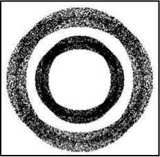
  a)

  
  
  
  
  

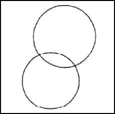
Figure 5.5: a) Cosine Cluster on DS6; b) BIRCH on DS6 and BIRCH. From these results, it is evident that Cosine Cluster is very powerful in handling any type of sophisticated patterns.

a)

Figure 5.6: a) Cosine Cluster on DS8; b) BIRCH on DS8

table i. required time (in seconds) for the clustering approaches.

No. of Data	DS1 100,000	DS2 100,000	DS3 100,000	DS4 60,266
CLARANS	1232.0	1093.0	1089.4	258.3
BIRCH	56.0	49.7	49.5	11.7
COSINE CLUSTER	4.41	4.34	4.40	1.22

c)    Cosine Cluster vs Wave Cluster

Properties of testing Environment

Processor – Intel® Core(TM) i3 CPU M380 @ 2.53GHZ

RAM – 4.00 GB (2.92 GB usable)

System Type – 32-bit Operating System

TABLE II. R equired time ( in seconds ) C osine C luster vs . W ave CLUSTER APPROACHES.

No. of Data	DS1 100,000	DS2 100,000	DS3 100,000	DS4 60,266
Wave Cluster	4.56	4.38	4.50	1.35
Cosine Cluster	4.41	4.34	4.40	1.22

Table II shows the slightly difference in performance between Cosine Cluster (The proposed algorithm) and Wave Cluster. It shows that Cosine Cluster better than Wave Cluster in performance .

• VI. conclusion

In this paper, the clustering approach Cosine Cluster is presented. It applies cosine transform on the spatial data feature space which helps in detecting arbitrary shape clusters at different scales. It is a very efficient method with time complexity of O(N), where N is the number of objects in the database, makes it especially attractive for large databases. Cosine Cluster is insensitive to the order of input data to be processed. Moreover, it is not affected by the outliers and can handle them properly and the difference on performance with Wave Cluster is shown above.