Coupling Perceptron Convergence Procedure with Modified Back-Propagation Techniques to Verify Combinational Circuits Design

Published Online May 2015 in MECS

Using parallel processing systems can help to overcome the limitations caused by a single processor system [1, 2]. For this reason, many of the Computer Aided Design (CAD) researchers are motivated toward using the parallel processing systems [3, 4].

Neural Networks can be considered as a complete different method of parallel processing, which are built up of huge interconnections of analog computing elements that cooperatively works to establish a solution to the problem [5].

Human brain is considered by many scientists as the last edge of exploration. Although they still lack the understanding of how the brain operates, many simplified neural network models have been proposed. Desiring to achieve human-like capabilities (such as voice recognition, medical diagnosis, vision, speech understanding, learning, etc.) [2] [6]. In a computer, researchers have been working for several years to implement neural network models into a new breed of computer system. These efforts have been successful, as commercial neurocomputers have become available recently. [7]

A neural network can be defined as "A cognitive information processing structure based upon models of brain function. In a more formal engineering context: a highly parallel dynamically system with the topology of a directed graph that can carry out information processing by means of its state response to continuous or initial input".[8]

Neural networks are constructed of processing elements (PEs, or neurons) that are interconnected via information channels called interconnects. A neuron is a two state processing element. The state 0 or 1, of a neuron is its activation value. In our model, the neurons are connected by links. Boolean operations are realized by specifying the thresholds for the neurons and the weights associated with these links. A typical neuron is shown in Fig. 1 [9].

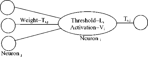
Fig. 1. Typical Neuron.

the weight T characterizes the link connecting neuron i to j. I and V are the threshold and activation ii value of neuron i. A state of neuron can be determined by calculating the weighted sum of the states of all the connected neighboring neurons and comparing this sum with its threshold. Typically, the neural networks are used for two classes of applications. [10] One class is the network performs constraint satisfaction tasks involving multiple constraints (combinatorial optimization) to find a consistent set of states. While in the other, the neural network learns from examples. The essential difference between the two applications is in the first class the network adjusts the states of the neurons to a given fixed set of connection strengths, while in the second the network adjusts the values of the connection strengths to give sample sets of neuron states. In the application of neural networks to hardware verification, we require both techniques, where the first one is used to verify the hardware design, and the other is used to teach the neuron the function of logic gates.

The gradient descent as employed by neural networks is a learning strategy which is analogous to the inductive techniques in symbolic AI. The perceptron convergence procedure, according to Rosenblatt, can guarantee the finding of a solution. This procedure is implemented to simulate the function of logic gates.

The process of teaching the perceptron was applied on two different computers and the required time and number of iterations are shown in Table 1.

Table 1. The required time and iterations for learning process.

Rate of convergence	Number of iterations	Learning time on Dell(N5010) i5 CPU Pentium 4 CPU
75%	45-55	0.30 – 0.35 sec.	1.0 – 1.5 sec.
90%	85 – 95	0.40 – 0.45 sec.	1.75 – 2.25 sec.

• II.    Modeling Logic Circuits by Neural Networks

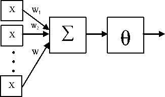
We used the Rosenblatt's Perceptron which is one of the earliest models of neural networks, to simulate the functions of logic gates. The Perceptron structure according to Rosenblatt is shown in Fig. 3, where the Perceptron has three major parts: the input vector, the weighted summation, and the threshold value [10].

• A.    Limitations of the Perceptron

While the convergence procedure guaranteed correct classification of linearly separable data, there were problems in which it does not supply such data (such as XOR problem) [2]. There is no one straight line which separates the decision surface of XOR problem as shown in Fig. 2( a).

(0,1)

(1,1)

(0,1)                              _(1,1)

Output

(0,0)                              (1,0)

OR

(b (0,1)

Output 0

(0,0)                               (1,0)

AND

(1,1)    (c)

Output 1

(0,0)                               (1,0)

XOR

Output

Fig. 3. Perceptron Structure.

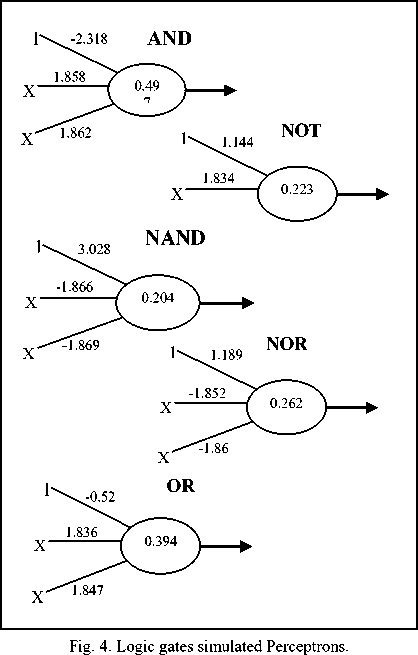
Other logic gates can be modeled by perceptron because their decisions surface are linearly separable as shown in Fig. 2( b, c). In order to overcome the problem of XOR gate, it can be built from other gates such as NAND gates. The main advantage of the perceptron model is the self-organization of the neuron and the ability to adapt itself for various numbers of inputs. Examples of learned perceptrons for the functions of two inputs logic gates are shown in Fig. 4.

(a)

Fig. 2. Logic Gates' decision surfaces.

The Perceptron can be trained on a sample of input/output pairs until it learns to compute the correct function of the specified logic gate. This training is done by the Perceptron Convergence procedure. This learning algorithm is a search algorithm that begins with a random initial state and finds a solution state. The search space is simply all the possible assignments of real values to the weights of the perceptron, and the search strategy used is the gradient descent.

• II.    A Technique for Hardware Verification

The emergence of neural networks brought about the researchers in the field of CAD systems to utilize the advantages of neural networks to improve the performance of such systems. The main aim of this research is to utilize the concepts of neural networks in the field of CAD, especially in the area of combinational circuit's verification.

The proposed verification algorithm is an attempt to transfer design automation techniques (in particular the design verification) from conventional computers to neurocomputers. We present the utilization of neural networks concepts in a field of hardware verification, in order to overcome the difficulties embedded within classical verification methods which require a thoroughly knowledge of algebra or high order logic to prove the correctness of the design. Since most the classical methods of formal verification are based on theorem proving, and a fully automated theorem proving system is very difficult to achieve.

The proposed verification algorithm is based on a modification of Rumelhart's Back-Propagation neural network which is designed for multi-layer feedforward nets (i.e. there are no feedback connections). This makes the proposed verification algorithm valid only for combinational circuits. The advantage given by the proposed algorithm is the predication of the component that causes the malfunction of the design, which provides an extra task over the classical methods of hardware verification.

• A. Back-Propagation neural network

The back-propagation neural network is one of the most important historical developments in neurocomputing. It is a powerful mapping network that has been successfully applied to a wide variety of problems ranging from credit application scoring to image compression [11]. The typical multi-layer feedforward neural network is shown in Fig. 5.

Output Layer

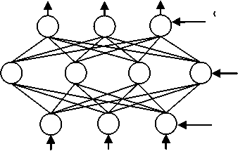
Hidden Layer

Input

Fig. 5. A typical multi-layer feed-forward neural network.

Like a perceptron, the learning algorithm of back-propagation neural network is supervised by a teacher. Hence, it begins with a random set of weights, then the network adjusts its weights each time it sees an input/output pair. Each pair requires two stages: a forward pass and a backward pass. The forward pass involves presenting a sample input to the network and letting activations flow until they reach the output layer. During the backward pass, the network's actual output is compared to the desired output, and error estimates are computed for the output units. The weights connected to the output units can be adjusted in order to reduce these errors. Then, the error estimates of the output units can be used to derive error estimates for the units in the hidden layers. Finally, errors are propagated back to the connections stemming from the input units. The following is the learning algorithm for back-propagation neural network:

Algorithm back-propagation (Input-Units A, Hidden-Units B, Output-Units C)

{ let x ,h ,ando , are the activation levels of the units in a, b, and c respectively, w1 , denotes the weights connecting Ai to B w2 , denotes the weights connecting bi to c

w1y = random (+ 0.1)

V i:i = 0 ••• A, Vj: j = 0 • B

w2y = random (+ 0.1)V i:i = 0 • B, Vj: j = 0 • C

Initialize the activation levels of the threshold units ( 6 ) as constant values.

V  (xi,Yi) : (xi,Yi) input/output pair and assign activation levels for the input units do:

h j =

1

A

- > wl,, • x, -0

1 + e ^ j j J

: h j is the activation function between A i to B i

1

j          -ГУ B w2ii • hi-б)

1 + e -    ’ i ^

: o j is the activation function between B i to C i

Let o j is the network's actual output and y j is the desired output

^{5 2} j = j ^{1 -} o jl y j ^- j

V j:j = 1 - C

: 52j are the errors in C j

51 = h, (1 -h,)-52, • w2n jj    j    j    j i=0

V j:j = 1 - B

: 51 j are the errors in B j

Let ( n ) , be the learning rate which has a function similar to the perceptron learning and its reasonable value is (0.35).

Aw2y = n • 52j • h

V i:i = 0 - B, V j:j = 1 - C

Aw1y = n • 51 у • xt

V i:i = 0 - A, V j :j = 1 - B

}

The algorithm above is a generalization of the Least Mean Square (LMS) algorithm. It uses a gradient technique to minimize a cost function equal to the mean square difference between the desired and actual net outputs. An essential component of the algorithm is the iterative process described in the algorithm that propagates the error terms required to adapt weights back from nodes in the output layer to the nodes in the lower layers.

Back-propagation suffers from several drawbacks. As a biological model, it is implausible; there is no evidence that synapses can be used in both directions. Even so, it does not seem readily believable that neurons can spread signal-activity levels or error signals using linear or nonlinear input/output functions depending on the direction of movement.

Nevertheless, from the point view of the computer engineering and connectionist modeling, biological implausibility is not a fundamental deficiency of back-propagation. Back-propagation's real limitations are those of all gradient-descent techniques, namely the possibility of getting stuck in local minima and a slow convergence rate.

• B.    The proposed algorithm

The proposed algorithm is based on the idea of representing each gate in the combinational circuit under consideration by a single perceptron, then connecting these perceptrons together in order to construct the multilayer network corresponding to the circuit under consideration. Then, apply a modified version of back-propagation algorithm to evaluate the output of the network (according to the design specification). We used perceptrons in order to eliminate the iterated steps of back-propagation algorithm that consumed in learning the behavior of the problem. That means if the design matches the specification, then only one forward pass will be applied for each input/output pair of the design specifications. In case of mismatch of the design with its specification, at this stage, the design is known to be incorrect. The extra task (predication part) over the classical verification methods will be performed, which is represented by a backward pass, performed in order to compute the errors in the neurons of each layer. These errors then are sorted in decreasing order, and the neuron with the highest error is considered as the most probable neuron (component) that causes the malfunction in the design. The proposed algorithm is given below:

Algorithm Developed-Advanced-Propagation (Input

Units A, Hidden-Units B, Output-Units C) {

let x ,h ,ando , are the activation levels of the units in a, b, and c respectively, w1 , denotes the weights connecting Ai to Bj w2 , denotes the weights connecting bi to cj w1y = random (+ 0.1)

• V    i:i = 0 - A, V j :j = 0 - B

w2_y = random ( + 0.1 )

• V    i:i = 0 - B, V j :j = 0 - C

Initialize the activation levels of the threshold units ( 6 ) as constant values.

V ( х;,У; ) : ( х;,У; ) input/output pair and assign activation levels for the input units do:

j             f v^a             : h is the activation

• -      W:• X: +9

• j           -I У B Wj • h + 9 I

• 1    + e - 1 j

• 10.    If (o j = y j )

• 11.    Continue

• 12.    ^O e = °У — ⁰,1 у j ^- o l )

  : O e

  
  

  are the errors in C j

  
  

• 13.    H e = h (1 - h, ) £ o , • W, ^J             i = 1

  H e

  
  

• 14.    Continue

• 15.    E j = max( O e , H_e )

• 16.    Node (j) has is the most probable neuron that causes the malfunction of the design, and so. Terminate to redesign.

function between B i to C i

Let o j is the network's actual output and y j is the desired output

are the errors in Aj, N is the number of the nodes in B

}

The proposed algorithm consists of two parts; steps 1-6 perform the simulation of the circuit under consideration. We used the perceptron convergence procedure to simulate the functions of standard logic gates, and the perceptrons resulting from this simulation could be saved in order to be used again in other circuits. Hence, we used the perceptron convergence procedure only once, and each time we need to simulate the circuit under consideration, we have the perceptrons corresponding to the gates of this circuit.

The simulation of logic circuits will be done by representing each gate in the circuit by its corresponding perceptron (neuron). Thus, a constructed network corresponds to the logic circuit under consideration.

The second part (steps 7 – 14), represents the verification part of the simulated circuit. As shown above, the verification method is based on the learning algorithm of back-propagation neural networks.

The verification part, in turn, is subdivided into two passes: forward pass and backward pass. In the forward pass (steps 7-11), an input/output pair, and the activations of the neurons will be propagated up to the output layer. The formula in step 3 propagates the activations from the input layer to the first hidden layer in the network. While the formula in step 8, is used to propagate the activation from the first hidden layer to the output layer. Notice, there is a difference between the formulas of steps 7 and 8, and the corresponding steps in the back-propagation algorithm, which is the addition of the threshold value in the proposed algorithm while it is subtracted in the back-propagation algorithm. This difference comes to increase the convergence of the produced output of the simulated network to the desired output (logic 1 or logic 0).now, the actual output will be computed, which is a real value results from the neural network corresponding to the circuit under consideration. If this real value is equal or greater than (0.5), it will be considered as logic 1, while if it is less than (0.5), then it is considered to be logic 0. So, if the actual output obtained from the network matches the desired output, then another pair will be chosen and the above process is repeated again. If the actual output does not match the desired one, this means that there is no matching between the desired specification of the circuit and its actual input/output pattern. Then, there is incorrect design to match the specifications.

In this case we have to perform the backward pass (steps 12-16), to compute the errors in the neurons and therefore to predict the gate that causes the malfunction in the design. The errors in the output layer will be computed using the formula in step 12, and then computing the errors in all the hidden layers up to the input layer using the formula in step 13 (this corresponds to error signals' propagation in back-propagation algorithm).

The prediction technique of the gate that causes the malfunction in the design will be performed by sorting the errors of the network neurons in decreasing order (step 15), and the first neuron in the sorted list is the most probable neuron (gate) that causes the malfunction in the design (the one needed to be changed in the design).

However, the prediction part of this algorithm is not so accurate, but it helps the designer to debug the design in less time than the time required without prediction phase. The inaccuracy of the prediction comes from the random numbers generated in step 1 that simulates the function of each logic gate. Simulating these gates by different sets of perceptrons (weight vectors and thresholds) will lead to different predictions in the design. Some of these sets were converged to correct prediction while others were diverged from it.

The complexity time required for this algorithm O ( k2ⁿ ) , where n represents the number of input variables, and ( 2ⁿ ) , represents the input/output pairs of the design specifications. The constant (k) represents the number of iterations performed by the algorithm for each input/output pair given to the network. Thus, the proposed verification algorithm requires exponential time. However, even with this disadvantage, the algorithm is still favorable compared with the time required in the classical methods of hardware verification which deals with theorem proving techniques to prove the correctness of the design.

• III.    Testing the Algorithm

For the purpose of testing, two examples are used to test the verification performance of the proposed algorithm. The first one is the well-known full adder circuit, while the second is a combinational circuit that performs a particular Boolean expression.

• A.    Full adder example

The correct design of the full adder is shown in Fig. 7( a), while the incorrect design is shown in Fig. 7( b). The corresponding neural network of the incorrect design is shown in Fig. 6 .Table 2 shows the forward part of the verification algorithm to compute the actual output. Table 3 shows the backward part of the algorithm to compute the errors of the neurons in the network.

The table also shows the sorted list of these neurons according to its error's values.

Notice that the prediction of the component that causes the malfunction diverges from the correct prediction (gate 4). However, the prediction is not so accurate, but it can help the designer in case of large circuits since this prediction can reduce the debugging time of the malfunction gate by at least 25% of the debugging time required by the designer in the classical methods of hardware verification.

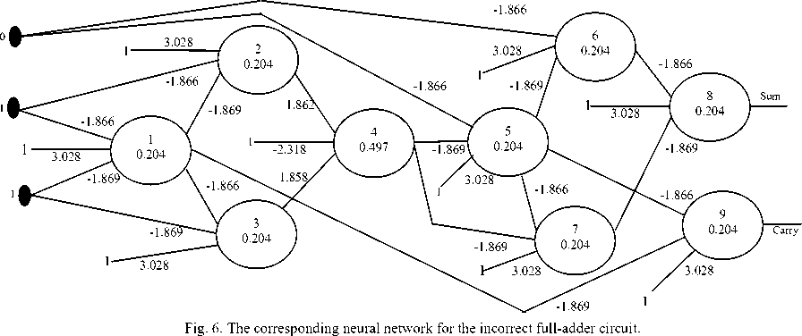
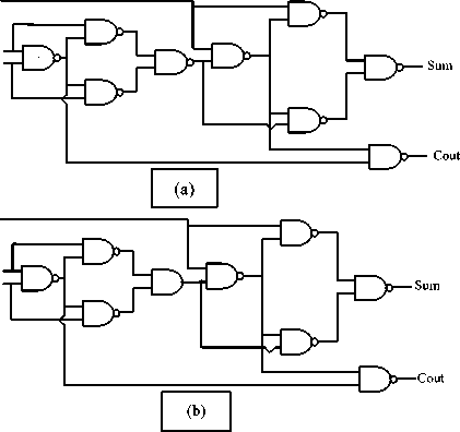
Fig. 7. Full adder circuit. (a) Correct design, (b) incorrect design.

Table 2. The activations of network neurons

Neuron	Weighted Sum	h &o
1	1(3.028)+ 1(-1.866)+1(-1.869)+0.204 = -0.503	0.377
2	1(3.028)+ 1(-1.866)+ 0.377(-1.869) + 0.204 = 0.66	0.66
3	1(3.028)+ 1(-1.869)+ 0.377(-1.866)+ 0.204 = 0.659	0.66
4	1(-2.318)+ 0.66(1.862)+ 0.66(1.858)+ 0.497 = 0.635	0.654
5	1(3.028)+ 0(-1.866)+ 0.654(-1.869)+ 0.204 = 2.01	0.882
6	1(3.028)+0(-1.866)+ 0.882(-1.869)+0.204 = 1.58	0.83
7	1(3.028)+ 0.882(-1.866)+ 0.654(-1.869) + 0.204=0.364	0.59
8	1(3.028)+ 0.83(-1.866)+ 0.59(-1.869) + 0.204= 0.581	0.641*
9	1(3.028)+ 0.882(-1.866)+ 0.377(-1.869) + 0.204= 0.88	0.707

(*): the activation value of neuron 8 is 0.641, which is greater than 0.5, which corresponds to logic 1. According to the correct design this value must be logic 0, which means a value less than 0.5.

Table 3.The errors in network neurons

Neuron	Error values in network neurons	Sorted list
9	0.707(1-0707)(1-0.707)= 0.0607	2
8	0.641(1-0.641)(0-0.641)= -0.148	9
7	0.59(1-0.59)[(-0.148)(-1.869)]= 0.0669	1
6	0.83(1-0.83)[(-0.148)(-1.866)]= 0.039	3
5	0.882(1-0.882)[(0.039)(-1.869)+(0.0669)(-1.866) + (0.0607)(-1.866)]= -0.0324	8
4	0.654(1-0.654)[(-0.0324)(-1.869) +(0.0669)(-1.866)]= -0.0145	7
3	0.66(1-0.66)[(-0.0145)(1.858)]= -0.006045	4
2	0.66(1-0.66)[(-0.0145)(1.862)]= -0.006058	5
1	0.377(1-0.377)[(-0.006058)(-1.869) + (-0.006045)(-1.866) +(0.0607)(-1.869)]= -0.0213	6

• B.    Boolean expression example

The second example deals with a combinational circuit that performs a particular function defined by the Boolean expression: f = ( x₂ + x₃ ) x₃ +— Х_гХ₄ .

Fig. 8( a, and b) shows the correct and the incorrect designs of the circuit. While Fig. 9s hows the corresponding neural network for incorrect design. Table 4 shows the forward part of verification algorithm to compute the actual output. Table 5, shows the backward part of the algorithm to compute the errors of neurons in the network. The table also shows the sorted list of the neurons according to their error values. The predication of the gate that causes the malfunction in this example is the gate 1.

From these two examples, the benefit of this verification algorithm is clearly obvious. The proposed algorithm can also be used with components other than the logic gates if they considered as combinational circuits (such as Decoders, Multiplexers, etc.).

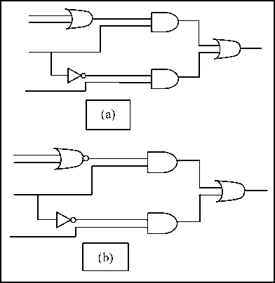
Fig. 8. Structure of function, (a) correct design, (b) incorrect design.

Hence such components are represented as boxes containing the logic gates that produce the functions of these components. The prediction part of the algorithm will be performed as usual except if the predicted neuron is included within the boundaries of a particular component, then the whole component will be considered as the most probable component that causes the malfunction of the design.

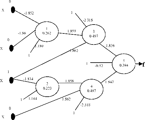
Fig. 9. The corresponding neural network of the design.

Table 4. the activations of network neurons

Neuron	Weighted Sum	h j &o j
1	0(-1.852)+0(-1.86)+1(1.189)+0.262 =1.451	0.81
2	1(-1.834)+1(1.144)+0.223 =-0.467	0.385
3	1(1.862)+0.81(1.858)+1(-2.318)+0.497 = 1.546	0.824
4	0(1.862)+0.385(1.858)+1(-2.318) +0.497= -1.106	0.249
5	0.824(1.836)+0.249(1.847)+1(-0.52) +0.394= 1.847	0.864*

Table 5. The errors in network neurons

Neuron	Error values in network neuron	Sorted list
5	0.864(1-0.864)(0-0.864) = -0.1015	5
4	0.249(1-0.249)[(-0.1015)(1.847)] = -0.035	4
3	0.824(1-0.824)[(-0.1015)(1.836)] = -0.027	3
2	0.385(1-0.385)[(-0.035)(1.858)] = -0.0154	2
1	0.81(1-0.81)[(-0.027)(1.858)] = -0.0077	1

• IV.    Conclusions

As a new trend in CAD systems, this work comes out with some conclusions:

• 1.    The verification algorithm is valid for combinational circuit only. This is due to the fact that the algorithm is based on the learning algorithm for back-propagation neural networks which is a feedforward network.

• 2.    The prediction technique in that is used in the algorithm can help the designer to locate the malfunction component easily and try to correct the design quickly.

• 3.    Although the complexity time of the algorithm is exponential, it is still work perfect for some small set of problems.

• 4.    The proposed algorithm does not need the classical proving theorem to prove the correctness of the hardware design.

• 5.    This work can pave the way to implement First-Order Predicate Logic as an HDL for the description and documentation of the hardware. Also, it can pave the way for using Temporal Logic to describe the timing relations among hardware modules (sequential circuits).

• 6.    Finally, this work can be considered as a step toward using Distributed CAD environments through the use of the parallel processing architecture specially the Neurocomputer architecture.

• [1]    Yangdong, D. " GPU Accelerated VLSI Design Verification" . in Proceeding of the IEEE 10th International Conference on Computer and Information Technology (CIT), 2010 . pp 1213-1218. 2010

• [2]    Raeisi, D.R. " MODELING AND VERIFICATION OF DIGITAL LOGIC CIRCUIT USING NEURAL NETWORKS" . in Proceeding of the 2005 IL/IN Sectional Conference . pp. 2005

• [3]    Li Da, X., W. Viriyasitavat, P. Ruchikachorn, and A. Martin," Using Propositional Logic for Requirements Verification of Service Workflow". IEEE Transactions on Industrial Informatics, vol. 8 no 3: pp. 639-646.2012

• [4]    Chang, P.-C., Y.-W. Wang, and C.-Y. Tsai," Evolving neural network for printed circuit board sales forecasting". Expert Systems with Applications, vol. 29 no 1: pp. 8392.2005

• [5]    Rabunal, J.R. and J. Dorado, Artificial Neural Networks in Real-life Applications : Idea Group Inc (IGI) - Technology & Engineering. 2006,

• [6]    Hosseini, S.B., A. Shahabi, H. Sohofi, and Z. Navabi. " A reconfigurable online BIST for combinational hardware using digital neural networks" . in Proceeding of the 15th IEEE European Test Symposium (ETS), 2010 . pp 139-144. 2010

• [7]    Ruehli, A.E. and G.S. Ditlow," Circuit analysis, logic simulation, and design verification for VLSI". Proceedings of the IEEE, vol. 71 no 1: pp. 34-48.2005

• [8]    Hassoun, S. and T. Sasao, Logic Synthesis and Verification , ed. T.S.I.S.i.E.a.C. Science. Vol. Vol. 654. 2003,

• [9]    Miller, R.K., Neural Networks . USA: Prentice-Hall Inc. 1990,

• [10]    Oldroyd, M., Optimisation of Massively Parallel Neural Networks , ed. F. Corporation. 2004,

• [11]    Chang, P.-C., C.-H. Liu, and C.-Y. Fan," Data clustering and fuzzy neural network for sales forecasting: A case study in printed circuit board industry". Knowledge-Based Systems, vol. 22 no 5: pp. 344-355.2009

  Authors’ Profiles

  
  
  

Raad Alwan is an associated prof. in Philadelphia University in Jordan. He completed his undergraduate from the University of Baghdad, Iraq. He finished his MSc. and PhD in University College Dublin and Trinity College Dublin, respectively. His research interests are algorithm analysis and design, data mining, logic design, and information retrieval.

Sami Eddi is an associated prof. in the University of Technology in Iraq. He completed his MSc degree in Al-Rafidain college of Sciences. His MSc and PhD degrees were from the University of Technology, Iraq. His research interests are computer networking, neural nets, and expert systems.

Baydaa Al-hamadani is an assistance prof. in Zarqa University in Jordan. She got her Bachelor degree from the University of Technology in Iraq in 1994, followed by MSc. in the same University in 2000. In 2011, she got her PhD from the University of Huddersfield in the UK from the School of Computing and Engineering. Her fields of interest are XML, compressing and retrieving information, ontology, and Bioinformatics.