CPU-Centric Evaluation of Lightweight CNNs for Four-Class Chest X-Ray Classification: Performance, Latency, and Quantization Limits

Published Online on October 8, 2026 by MECS Press

The volume of medical imaging is growing faster than the number of radiologists available to interpret it, transforming the automation of primary chest X-ray analysis from an academic pursuit into a practical necessity for healthcare systems. Deep learning methods, primarily convolutional neural networks (CNNs), have demonstrated expertlevel performance in this task [1,2], with several systems having already undergone clinical evaluation. However, the

This work is open access and licensed under the Creative Commons CC BY 4.0 License.

transfer of such models into routine clinical practice is limited not by recognition performance but by computational requirements: a typical solution assumes a graphics processing unit (GPU), the availability of which in district hospitals, mobile diagnostic units and field hospitals remains the exception rather than the rule.

A review of the literature reveals a systematic asymmetry in reporting. Studies reporting the highest performance metrics typically rely on high-capacity architectures such as VGG, ResNet, Xception, DenseNet and transformer-based models – or on ensembles of several such networks [2-5]. At the same time, the computational costs of these solutions are documented inconsistently: parameter counts are reported relatively often, operation counts only occasionally, and central processing unit (CPU) inference latency almost never. Consequently, engineers tasked with deploying these systems on target hardware are left without the empirical data required for model selection: published accuracy values give no indication of whether a model fits the available resource budget.

Concurrently, the computer vision community has developed a distinct class of lightweight architectures designed for resource-constrained environments – namely the MobileNet and EfficientNet families [6-8], alongside model compression techniques, among which post-training quantization is the most extensively documented [9-11]. While these approaches are widely adopted in general-purpose mobile applications, the open literature lacks a systematic evaluation of their efficacy in chest X-ray analysis based on direct CPU profiling rather than parameter-count proxies. Consequently, a fundamental practical question remains open: what is the actual diagnostic performance penalty associated with adopting a lightweight model, and is this trade-off acceptable?

Research over the past three years has begun to bridge this gap along two main directions. First, purpose-built lightweight networks now achieve competitive accuracy in four-class chest X-ray classification without relying on pretraining or model ensembles [12], edge-based classification pipelines for X-ray imagery have been developed [13], and recent surveys frame model evaluation in terms of accuracy per unit of computation rather than accuracy alone [14]. Second, the reliability of post-training quantization has come under scrutiny: benchmarking studies show that widely used post-training schemes are unreliable under worst-case conditions [15], layer-sensitivity analyses identify MobileNetV3 in particular as degrading under uniform quantization due to weight outliers in its depthwise and squeeze-and-excitation blocks [16], and surveys document quantization-aware training (QAT) as the necessary remedy when post-training quantization fails on compact architectures [17]. What remains absent – and what this study explicitly addresses – is a unified evaluation in which candidate architecture computational costs, measured CPU latencies on identical hardware, and the empirical quantizability of lightweight models are reported together under a single, standardized protocol.

This establishes the primary rationale for the present work. Rather than pursuing a further accuracy gain by constructing yet another model, the aim is to quantify the relationship between diagnostic performance and computational resource consumption. The goal is not to identify a single best model, but to derive an empirically measured functional dependence that enables an informed choice of architecture tailored to the target hardware.

The aim of this work is the experimental justification of the choice of a lightweight neural network model for chest X-ray classification that is suitable for deployment on resource-constrained hardware without a graphics accelerator, using the ratio of diagnostic performance to computational cost as the selection criterion. The following objectives were defined:

• 1)    to compute, with a single tool, the computational cost of widely used neural network architectures and to quantify the gap between them;

• 2)    to establish a reproducible experimental protocol, identical for all models under study, and a protocol for measuring resource characteristics on the central processing unit (CPU);

• 3)    to train a heavy baseline and lightweight models under this protocol and to measure their performance metrics and computational cost;

• 4)    to evaluate the effectiveness of post-training quantization as a means of further reducing resource requirements;

• 5)    to verify the robustness of the conclusions on an independent dataset and to analyze the localization of the features the model relies on;

• 6)    to formulate a justified deployment recommendation and to define the limits of applicability of the results obtained.

2.    Computational Cost of Neural Network Architectures 2.1.    Analysis of Existing Approaches

• 2.2.    Differences from Existing Evaluation Work

• 2.3.    Computation Methodology and Results

The object of the study is the process of automated chest X-ray classification by means of deep learning under resource-constrained conditions. The subject of the study comprises lightweight convolutional neural network architectures, methods for their quantization, and techniques for measuring the ratio of diagnostic performance to computational complexity.

Chest X-ray classification is one of the most extensively studied tasks in medical computer vision. The CheXNet model based on DenseNet121 [2] set a methodological template for subsequent work, and the COVID-19 pandemic gave rise to a large body of research in which ResNet, VGG, Xception, and their combinations were applied to discriminate between COVID-19, pneumonia and the normal state [3-5]. The accuracy values reported in these studies typically exceed 0.95, with the highest values achieved by ensembles of several pretrained neural networks.

A feature common to these studies is that the computational cost of the solution is not part of the evaluation framework. Models are compared along a single dimension, performance, so the natural winner is invariably the heaviest configuration. Resource characteristics, where reported at all, are limited to the parameter count, which on its own determines neither the speed nor the deployability of a model: a model with few parameters may execute more operations than a model with many, and CPU latency additionally depends on the structure of the computational graph and on the properties of the runtime environment. For this reason, the present work measures not a single quantity but the complete resource profile.

The present study differs from existing evaluation work in three respects. First, studies that propose a lightweight chest X-ray classifier normally report accuracy and parameter count for one proposed network [12], and where deployment is addressed, the evaluation is framed around a chosen target device rather than around a cost axis shared by several architectures [13]; here the cost of 15 architectures is computed with a single tool and the performance of a subset is measured under a single training protocol, so performance and cost remain commensurable across models. Second, surveys of lightweight deployment enumerate compression techniques and hardware options [14] but do not report end-to-end CPU latency for medical imaging models under a stated measurement protocol; the protocol of Section 3.3 is specified here in full, including thread count, warm-up, repetition count and the statistic reported. Third, the literature on quantization reliability establishes that post-training quantization can fail [15-17] but does not report such a failure for a medical imaging task; the collapse of MobileNetV3-Small documented in Section 4.3, together with the full set of remediation attempts that did not resolve it, is, to the authors' knowledge, the first such case reported for chest X-ray classification.

The computational cost of 15 architectures was computed for an input resolution of 224×224 using the ptflops library [18], the same tool with which the experimental models are profiled later, which makes the review and the results methodologically consistent. Weights are not loaded in this procedure: only the structure of the graph is analyzed.

The reconciliation of units deserves separate attention. The tool used counts multiply-accumulate operations (MACs), whereas in the chest X-ray literature these values are frequently reported as floating-point operations (FLOPs). Since one MAC corresponds to two floating-point operations, the discrepancy is exactly twofold: our computation yields 2.856 GMACs for InceptionV3, i.e., 5.712 GFLOPs, and it is the value of approximately 5.7 that appears in review papers. Table 1 therefore reports both columns with explicit headings. The same reconciliation applies to ResNet50, for which the present computation yields 4.132 GMACs, i.e., 8.265 GFLOPs; the figure of approximately 4.1 that is frequently quoted for this architecture as a FLOP count is in fact a MAC count and conflating the two understates the cost of the baseline twofold. Every value in Table 1 was additionally cross-checked against an independent counting method, with the largest deviation being 1.05%.

Table 1. Computational Cost of Widely Used Architectures at an Input Resolution of 224×224

Architecture	Parameters, M	GMACs	GFLOPs	Class
VGG19	143.67	19.689	39.378	Heavy
ViT-B/16	86.57	17.606	35.212	Heavy
VGG16	138.36	15.523	31.046	Heavy
ResNet101	44.55	7.865	15.730	Heavy
Xception	22.86	4.599	9.199	Heavy
ResNet50	25.56	4.132	8.265	Heavy
ConvNeXt-Tiny	28.59	4.488	8.977	Heavy
DenseNet121	7.98	2.900	5.800	Medium
InceptionV3	23.83	2.856	5.712	Medium
EfficientNet-B0	5.29	0.410	0.820	Light
SqueezeNet 1.1	1.24	0.360	0.720	Light
MobileNetV2	3.50	0.320	0.641	Light
ShuffleNetV2-x1.0	2.28	0.152	0.305	Light
MobileNetV3-Small	2.54	0.061	0.122	Light
TinyCNN (custom)	0.14	0.061	0.123	Light

The computational gap between the heaviest architecture (VGG19) and the lightest one amounts to a factor of 323, and in terms of parameter count to more than 1000 times. The difference in published accuracy on chest X-ray tasks, by contrast, is measured in single percentage points. Adding the two most recent architectures named above did not move either end of the range: ShuffleNetV2-x1.0, at 0.152 GMACs, is cheaper than every heavy network but still 2.5 times more expensive than the lightest entry. This ratio alone casts doubt on the default choice of heavy architectures and gives rise to the hypothesis of the study: the final fraction of accuracy costs a disproportionate amount of computation, and consequently, a configuration exists that is practically equivalent in performance while being substantially cheaper to operate.

3.    Experimental Methodology 3.1.    Datasets

The primary dataset is the COVID-19 Radiography Database [3, 4]: 21,165 PNG images of 299×299 pixels in four classes, namely normal (10,192 images, 48.2%), lung opacity (6,012 images, 28.4%), COVID-19 (3,616 images, 17.1%), and viral pneumonia (1,345 images, 6.4%). A stratified 80/10/10 split was performed with a fixed random seed of 42, yielding 16,933, 2,116 and 2,116 images, respectively. The imbalance ratio between the largest and the smallest class is 7.6, and the macro-averaged F1 score (macro-F1) was therefore adopted as the primary metric instead of accuracy, which, on such a distribution, systematically overestimates performance in favor of the dominant class. The imbalance was compensated by class weights in the loss function; weighted sampling was deliberately not applied in order to avoid a double correction.

The external dataset is Chest X-Ray Images (Pneumonia) [5]: 5,856 images in two classes. It was not used in training and was employed solely to verify the transfer of the resulting models to independent data.

The preprocessing pipeline is identical for every architecture and consists of the following steps. (1) Each file is read and converted to a single-channel 8-bit grayscale representation; the sources are lossless PNG, so no lossy compression artifacts are introduced. (2) The image is resized from its native 299×299 to a 256×256 on-disk cache by bilinear interpolation, materialized once so that every architecture reads byte-identical input. (3) At training time, a random resized crop to 224×224 is taken with a scale range of 0.8–1.0 and an aspect-ratio range of 0.9–1.1, followed by horizontal flipping with probability 0.5, rotation within ±10° and brightness and contrast jitter of 0.2; at validation and test time, the cached image is resized directly to 224×224 with bilinear interpolation and antialiasing and no augmentation is applied. (4) The single grayscale channel is replicated three times, because the pretrained backbones expect three input channels. (5) Values are scaled to the interval [0,1] and normalized channel-wise with the ImageNet statistics, namely means of 0.485, 0.456 and 0.406 and standard deviations of 0.229, 0.224, and 0.225. Vertical flipping is deliberately excluded, an inverted thorax being anatomically impossible.

• 3.2.    Training Protocol

  All architectures were trained under a unified protocol, which is the principal condition for a valid comparison: the only variable is the model itself. The configuration comprised the AdamW optimizer with a learning rate of 3 X 10^-4 and weight decay of 10^-4, a cosine learning rate schedule with three warm-up epochs, up to 20 epochs, early stopping on validation macro-F1, label smoothing of 0.05 and a batch size of 32. The augmentations were random resized cropping (0.8–1.0), horizontal flipping, rotation within ±10° and brightness and contrast jitter of 0.2. The checkpoint with the best validation macro-F1 was retained. The initialization differs by architecture and is stated explicitly because it governs the achievable performance: ResNet50 was initialized with the torchvision ImageNet-1k V2 weights, while EfficientNet-B0 and MobileNetV3-Small were initialized with the corresponding ImageNet-1k V1 weights, in every case with the classification head replaced by a four-way head trained from scratch, whereas TinyCNN has no pretrained counterpart and was trained from random initialization throughout. The random seed is separated into two independent controls. The data split uses a seed of 42 in every run without exception, so that all configurations are evaluated on exactly the same 2,116 test images, and paired significance tests are admissible. The training seed, which governs weight initialization, data order and augmentation, takes the values 42, 1337 and 2024, so each of the four architectures was trained three times under an otherwise identical protocol. Performance figures are therefore reported as mean and standard deviation over three runs; the ablation points of Section 4.7 were trained once and are marked accordingly. The software environment was PyTorch 2.13.0 with torchvision 0.28.0.

• 3.3.    Resource Measurement Protocol

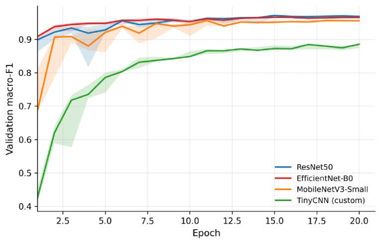
Fig. 1. Validation macro-F1 per epoch under the unified training protocol. Line: median over three training seeds; band: min–max.

The dip of ResNet50 at the fourth epoch, visible in every seed (Fig. 1), corresponds to the transition from the warmup phase to the cosine decay schedule; it does not affect the reported results, since the best checkpoint is retained. The lightweight models exhibit a markedly more stable trajectory, which is a practically relevant side result: under a limited budget for hyperparameter tuning, they are less sensitive to its imprecision.

TinyCNN is specified in full in Table 2, since no published reference defines it. It comprises a strided stem convolution followed by five depthwise-separable blocks and a linear classifier, for a total of 0.135 M parameters; spatial reduction is performed by a stride of two in the first convolution of a block, so the network contains no separate pooling layers apart from the final global average pooling. Every convolution is followed by batch normalization and a hard-swish activation, and convolutions carry no bias term because the subsequent batch normalization makes it redundant.

Table 2. Architecture of the Custom TinyCNN Network (Input 3×224×224, Four Output Classes)

Stage	Operation	Kernel / Stride	Output Channels	Output Size
Stem	Conv2d, BatchNorm, Hardswish	3×3 / 2	32	112×112
Block 1	Depthwise 3×3, BN, Hardswish; Pointwise 1×1, BN, Hardswish	3×3 / 2, 1×1 / 1	64	56×56
Block 2	Depthwise 3×3, BN, Hardswish; Pointwise 1×1, BN, Hardswish	3×3 / 2, 1×1 / 1	128	28×28
Block 3	Depthwise 3×3, BN, Hardswish; Pointwise 1×1, BN, Hardswish	3×3 / 1, 1×1 / 1	128	28×28
Block 4	Depthwise 3×3, BN, Hardswish; Pointwise 1×1, BN, Hardswish	3×3 / 2, 1×1 / 1	256	14×14
Block 5	Depthwise 3×3, BN, Hardswish; Pointwise 1×1, BN, Hardswish	3×3 / 1, 1×1 / 1	256	14×14
Head	Global average pooling, Dropout p = 0.2, Linear	–	4	1×1

Training was performed on the graphics processing unit of an Apple M3 Pro system-on-a-chip, whereas the resource profile was measured strictly on the central processing unit through the Open Neural Network Exchange (ONNX) Runtime 1.29.0 [19] with the CPUExecutionProvider. This separation is not a contradiction, since the object of evaluation is the cost of inference in operation rather than the cost of a one-off training run.

The measurement parameters were as follows: a batch size of 1, since the clinical scenario involves processing a single image rather than a batch; 1 and 4 threads measured separately; sequential execution mode; full graph optimization; 20 warm-up runs; and 200 measurements in each of three independent sessions. The median and the 95th percentile are reported rather than the mean, because the latency distribution is asymmetric, and the mean is sensitive to isolated outliers. The FP32 and INT8 configurations were measured in the same runtime environment under identical settings.

During the measurements, the background CPU load was 2.8–18%. The ratios between models are unaffected in any case, since all configurations were measured under identical conditions; for specific target hardware the absolute values should be remeasured, while the protocol itself requires no modification.

• 3.4.    Problem Formalization and Efficiency Indicator

Model selection is formalized as a multi-criteria problem of maximizing diagnostic performance over the set of configurations considered flmacro(m) ^ max,m e M                                 (1)

subject to constraints on computational resources

C(m) < C_max,     L(m) < L_max,     S(m) < S_m ax                         (2)

where m is the set of configurations considered, C (m) is the computational complexity expressed in GFLOPs, that is, twice the MAC count reported in Table 1, L(m) is the CPU inference latency, S(m) is the on-disk model size, and Cmax, Lmax, and Smax constitute the resource budget of the target hardware. To rank configurations by the performance-to-cost ratio, a scalar efficiency indicator is introduced x    f1macro(m)

^E(m) = ——                           (3)

C (m)

Indicator (3) is measured in units of F1macro per GFLOP, and every efficiency value quoted in Section 4.1 uses that unit; the ratio between two configurations is of course independent of whether MACs or FLOPs are used, since the conversion factor cancels. The solution of problem (1)-(2) is not a single model but a set of Pareto-optimal configurations; the choice within this set is determined by the resource budget, while indicator (3) allows configurations located in different regions of the Pareto front to be compared.

4.    Experimental Results 4.1.    The Performance to Computational Resources Trade-off

Of the 15 architectures costed in Table 1, four were selected for training. The selection samples the cost axis at four points rather than attempting to be exhaustive, because the research question concerns the shape of the performance-to-cost relation and not the ranking of individual networks. ResNet50 was taken as the heavy baseline: it is the most frequent baseline in the chest X-ray literature, so any resource saving has to be quoted against it. MobileNetV3-Small represents the lightweight state of the art and is the cheapest architecture in Table 1 for which pretrained ImageNet weights are available. EfficientNet-B0 was added as a second, more recent lightweight architecture occupying the intermediate region of the cost axis, so that the recommendation of Section 5 is tested against a competitor rather than only against the heavy baseline. TinyCNN defines the lower bound of the axis, its parameter count being two orders of magnitude below the baseline. The four together span the full 69-fold range of computational cost present in Table 1 while keeping the number of full training runs, and hence the energy cost of the study, proportionate to its aim. Architectures of intermediate cost, in particular MobileNetV2, SqueezeNet 1.1, ShuffleNetV2-x1.0, and ConvNeXt-Tiny, are costed in Table 1 but were not trained; that restriction is stated as a limitation in Section 6.

Each of the four was evaluated in two numerical-format configurations, namely 32-bit floating point (FP32) and quantized 8-bit integer (INT8). ResNet50 is used in the form specified in [20], and TinyCNN as specified in Table 2. The aggregated experimental data are given in Table 3.

Table 3. Performance and Computational Cost of the Evaluated Configurations (performance as Mean ± STD over three training seeds)

Indicator	ResNet50 FP32	ResNet50 INT8	EfficientNet-B0 FP32	EfficientNet- B0 INT8	MobileNetV3- Small FP32	MobileNetV3- Small INT8	TinyCNN FP32	TinyCNN INT8
Parameters, M	23.52	23.52	4.01	4.01	1.52	1.52	0.14	0.14
Computation, GMACs	4.13	4.13	0.41	0.41	0.06	0.06	0.06	0.06
Computation, GFLOPs	8.26	8.26	0.82	0.82	0.12	0.12	0.12	0.12
Model size, MB	89.63	22.91	15.30	4.66	5.81	1.78	0.52	0.19
Accuracy	0.9622 ±	0.9579 ±	0.9576 ±	0.4876 ±	0.9516 ±	0.1752 ±	0.8900 ±	0.8817 ±
	0.0029	0.0029	0.0052	0.1169	0.0015	0.0059	0.0040	0.0005
Macro–F1	0.9681 ±	0.9629 ±	0.9624 ±	0.5311 ±	0.9557 ±	0.0887 ±	0.8933 ±	0.8882 ±
	0.0021	0.0029	0.0064	0.0954	0.0016	0.0135	0.0030	0.0005
Efficiency, macro-F1 per GFLOPs	0.117	0.117	1.18	0.65	7.98	0.74	7.29	7.25
ROC-AUC	0.9931 ±	0.9929 ±	0.9944 ±	0.9136 ±	0.9921 ±	0.5615 ±	0.9803 ±	0.9799 ±
	0.0003	0.0008	0.0015	0.0337	0.0013	0.0224	0.0016	0.0014
Latency, 1 thread, ms	84.13	23.52	20.77	6.48	4.36	1.34	2.22	1.23
Latency p95, ms	84.69	25.24	21.04	6.65	4.44	1.35	2.24	1.27
Latency, 4 threads, ms	26.19	7.09	6.33	3.05	1.53	0.78	0.75	0.60
Throughput, img/s	11.9	42.5	48.2	154.3	229.4	745.4	450.3	814.2
Peak RAM, MB	214	144	130	97	83	77	75	71
Configuration State	Operation al	Operational	Operational	Failed	Operational	Failed	Operational	Operational

The result obtained is as follows: MobileNetV3-Small in the FP32 representation trails the heavy baseline by only 1.24 percentage points of macro-F1 (0.9557 versus 0.9681, averaged over three training seeds) while requiring 69 times fewer operations (0.06 versus 4.13 GMACs, equivalently 0.12 versus 8.26 GFLOPs), 19.3 times lower latency on a single CPU core (4.36 versus 84.13 ms per image), a 15.4 times smaller on-disk footprint (5.81 versus 89.63 MB), and 2.6 times less random-access memory (83 versus 214 MB). The efficiency indicator (3) for these configurations equals 7.98 versus 0.117 macro-F1 per GFLOP, a difference of a factor of 68.

The gap is small, but it is not noise. The standard deviation of macro-F1 across training seeds is 0.21 percentage points for ResNet50 and 0.16 for MobileNetV3-Small, so the difference between the two architectures is roughly six times the spread of either. Two independent tests are reported in Table 4 because they answer different questions. A paired t-test across the three seeds describes how far the result depends on the randomness of training; with three observations its power is negligible, so it is offered as a description rather than as proof. A paired bootstrap over the 2,116 test images, with 10,000 resamples drawn on indices shared by both models, and an exact McNemar test on the same images are the actual tests of significance; they are admissible only because the data split is identical for every configuration. The Holm correction is applied within each family of comparisons separately, since the four families answer four different questions and pooling them would penalize the central claim for the exploratory ones. The difference between the baseline and the lightweight architecture is significant under both levels, whereas the difference between MobileNetV3-Small and EfficientNet-B0 is not (p = 0.77), although EfficientNet-B0 costs 6.8 times more computation and 4.8 times more latency. The loss that quantization inflicts on ResNet50 and on TinyCNN is not significant after correction, so for those two models INT8 is free within statistical error.

Table 4. Significance of the Principal Comparisons (macro-F1 unless stated otherwise, Holm correction within each family)

Comparison	Level	Δ, pp	95% CI	Test	p	p (Holm)
ResNet50 vs. MobileNetV3-Small	Across seeds	1.24	[0.84, 1.63]	Paired t	0.0054	0.0054
ResNet50 vs. MobileNetV3-Small	Paired test set	1.12	[0.25, 1.99]	Bootstrap	0.0106	0.0106
ResNet50 vs. MobileNetV3-Small (Accuracy)	Paired test set	1.09	-	McNemar	0.0165	0.0165
MobileNetV3-Small vs. TinyCNN	Paired test set	6.11	[4.76, 7.50]	Bootstrap	0.0001	0.0001
MobileNetV3-Small vs. EfficientNet-B0	Paired test set	-0.11	[-0.89, 0.65]	Bootstrap	0.7726	0.7726
ResNet50 FP32 vs. INT8	Paired test set	0.31	[-0.04, 0.69]	Bootstrap	0.0848	0.3392
EfficientNet-B0 FP32 vs. INT8	Paired test set	50.42	[48.40, 52.58]	Bootstrap	<0.0001	0.0007
MobileNetV3-Small FP32 vs. INT8	Paired test set	85.59	[83.87, 87.17]	Bootstrap	<0.0001	0.0007
TinyCNN FP32 vs. INT8	Paired test set	0.74	[0.14, 1.35]	Bootstrap	0.0174	0.0870

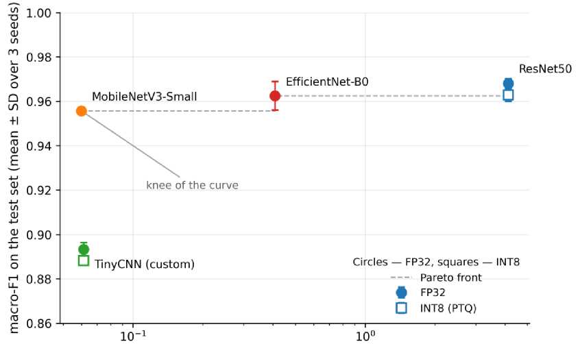
Computational complexity, GM AC (log scale)

Fig. 2. The performance to computational complexity trade-off. Error bars: SD over three training seeds

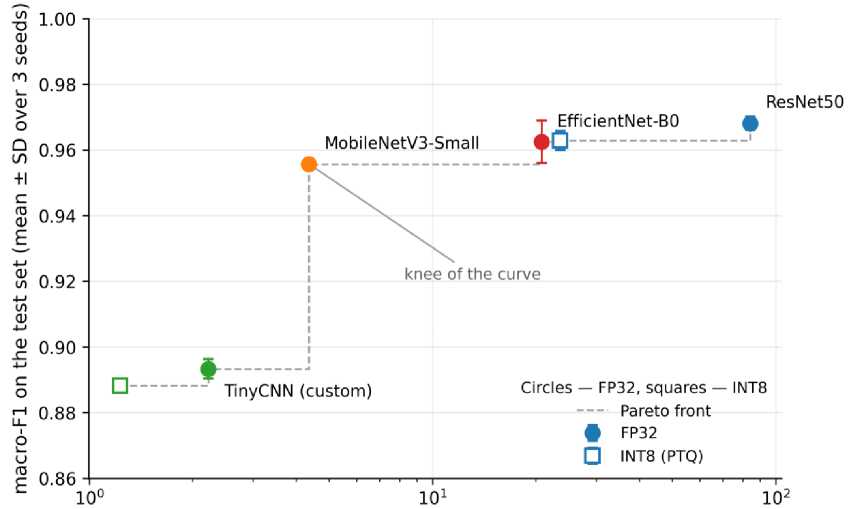
CPU latency, ms per image (1 thread, log scale)

Fig. 3. The performance to CPU inference latency trade-off. Error bars: SD over three training seeds

The dependence shown in Fig. 2. and Fig. 3. exhibits a pronounced knee located precisely at MobileNetV3-Small FP32: before this point, an increase in computation yields a substantial gain in performance, whereas beyond it the gain is disproportionately small. Four configurations are Pareto-optimal in the macro-F1 to latency coordinates: TinyCNN INT8, TinyCNN FP32, MobileNetV3-Small FP32, and ResNet50 FP32. ResNet50 INT8 lies on the Pareto front in the performance to latency coordinates but is Pareto-dominated in terms of computational complexity. The remaining configurations are Pareto-dominated and are not considered further.

The practical significance of this result lies in a quantitative reassessment of the computational price of an accuracy gain. Moving from MobileNetV3-Small to ResNet50 improves macro-F1 by 0.0124 at the cost of 80 additional milliseconds per image; for a throughput of 1,000 images per day, this is the difference between 4 seconds and 1.4 minutes of CPU time, and on weaker hardware, the difference between an acceptable and an unacceptable system response.

• 4.2.    Effectiveness of Post-Training Quantization

• 4.3.    Quantization Failure of the Squeeze-and-Excitation Architectures

  Two of the four architectures do not survive post-training quantization, and both fail in all three runs. For MobileNetV3-Small macro-F1 falls from 0.9557 to 0.0887 and the area under the receiver operating characteristic curve (ROC-AUC) to 0.5615, that is, to near chance level; the model returns an almost constant class, and on the external dataset this manifests itself as a specificity of 0.000 at a recall of 0.998, meaning that it labels every image as pathological. For EfficientNet-B0 macro-F1 falls from 0.9624 to 0.5311 at a specificity of 0.002, but ROC-AUC is retained at 0.9136: the ranking of the images largely survives, and it is the decision thresholds that are destroyed. The failure is therefore graded rather than binary, and the outcome is presented as a self-contained finding of the study rather than as a measurement artifact.

In order to further reduce memory consumption and to accelerate CPU inference, post-training quantization (PTQ) was applied. The conversion of weights and activations to an 8-bit integer representation was performed in the quantize-dequantize (QDQ) format with per-channel weight scaling and percentile calibration at the 99.999 percentile on a calibration subset of 300 training images. The resulting compression and the corresponding changes in diagnostic performance are given in Table 5.

Table 5. Effect of Post-Training Quantization to INT8 against the Structural Signature of Each Architecture

Architecture	Depthwise	SE Blocks	Activation	Mul Nodes	Δ macro-F1, pp	Collapses	Compression	Speed-up
ResNet50	No	No	ReLU	0	-0.52	0/3	3.91x	3.58x
EfficientNet-B0	Yes	Yes	SiLU	65	-43.13	3/3	3.28x	3.20x
MobileNetV3-Small	Yes	Yes	HardSwish	9	-86.70	3/3	3.26x	3.25x
TinyCNN (custom)	Yes	No	HardSwish	0	-0.51	0/3	2.72x	1.81x
TinyCNN w16	Yes	No	HardSwish	0	+0.50	0/1	1.67x	1.45x
TinyCNN w48	Yes	No	HardSwish	0	-0.25	0/1	3.19x	2.06x
TinyCNN d3	Yes	No	HardSwish	0	-0.66	0/1	2.25x	1.73x

For ResNet50, quantization proved to be the most effective single optimization: a 3.91-fold reduction in size and a 3.58-fold speed-up at the cost of only 0.52 percentage points of macro-F1, a loss that is not significant after correction (Table 4). Percentile calibration substantially outperformed the standard MinMax scheme (0.9654 versus 0.9547 at training seed 42), preserving an additional 1.07 percentage points of macro-F1 solely through the choice of quantization ranges.

Eight post-training quantization configurations, grouped into six remediation strategies, were examined for MobileNetV3-Small, and none produced an operational model (Table 6). Only three of the eight vary the calibration method; the remaining five vary weight granularity, range reduction, activation representation, node exclusion and operator scope. The sweep was run at training seed 42, at which the main pipeline gives a macro-F1 of 0.1014 against the three-seed mean of 0.0887 reported above; the value of 0.0948 in Table 6 is an independent requantization of the same checkpoint under the same setting but with a separately drawn calibration subset. These differences carry no interpretation, since all of them describe a model that has collapsed to a near-constant output, and no configuration in Table 6 comes within 85 percentage points of the corresponding FP32 macro-F1. It was additionally verified that the graph preprocessing stage is not the cause, the logits of the FP32 model before and after that stage coinciding bit-exactly.

Table 6. Post-Training Quantization Configurations Examined for MobileNetV3-Small (Training Seed 42)

Remediation Strategy	Configuration	Macro-F1
Calibration Method	MinMax	0.0745
Calibration Method	Percentile 99.999 (re-quantization)	0.0948
Calibration Method	Entropy	0.0745
Weight Granularity	Per-channel scaling disabled	0.0745
Range Reduction	Reduced range enabled	0.0745
Activation Representation	Signed INT8 instead of unsigned	0.1022
Node Exclusion	Squeeze-and-Excitation multiplication nodes excluded	0.0745
Operator Scope	Convolutional and matrix nodes only	0.0745
Reference	FP32, no quantization	0.9573

The cause is architectural rather than implementation-related, and the four architectures form a controlled 2×2 design that separates the candidate explanations (Table 5). Depthwise separable convolutions are not the cause: the TinyCNN family consists of nothing else and quantizes without loss in six configurations out of six. The hard-swish activation is not the cause either, since TinyCNN uses it throughout and does not degrade, while EfficientNet-B0 collapses under a different activation. What the two failing architectures share, and what no surviving architecture has, is a squeeze-and- excitation block placed after a depthwise convolution. In the exported graph such a block leaves a channel-wise multiplication node, and the count of those nodes separates the sample exactly: every architecture with zero of them survives, and both architectures with a non-zero count fail in three runs out of three. The predictor is thus a number that can be read off the static graph before any training, rather than a qualitative property that has to be known in advance. It predicts the fact of the failure but not its severity, which differs by an order of magnitude between the two cases. This is consistent with the sensitivity of depthwise separable convolutions and of channels with dynamic reweighting to posttraining quantization reported in the literature [10, 11, 15, 16, 21]: the activation ranges of individual channels in such blocks differ by orders of magnitude, so a single quantization scale inevitably destroys part of the signal. The standard remedy is quantization-aware training [17], which was not implemented within this study.

One further regularity is worth recording because it is usable as an acceptance criterion in its own right. The two collapsed configurations are not merely poor; they are unstably poor: the standard deviation of macro-F1 across seeds is 0.0954 for EfficientNet-B0 INT8 and 0.0135 for MobileNetV3-Small INT8, against 0.0005 to 0.0029 for every configuration that survives quantization. Instability of INT8 performance across seeds therefore signals the failure by itself, before any comparison with the FP32 model. The collapse is visible in the calibration as well: expected calibration error rises from 0.085 to 0.685 for MobileNetV3-Small and from 0.083 to 0.247 for EfficientNet-B0, while it is unchanged for the models that quantize correctly, and the agreement between FP32 and INT8 decisions falls to 18.5% and 40.6% respectively, against 97–99% elsewhere. For a decision-support system, this matters more than the loss of accuracy alone: the model does not merely become wrong; it becomes confidently wrong.

The MobileNetV3-Small INT8 configuration was excluded from the Pareto analysis and from the recommendations. This is essential: in terms of formal resource indicators, it is the most attractive configuration in the entire study, having the smallest size and the lowest latency, precisely because it performs no useful work. The practical implication, which is of substantial value for engineering practice, is that the quantizability of a lightweight model must not be assumed by analogy: it has to be verified by measuring performance after quantization. The risk is highest exactly where the resource gain is most desirable.

• 4.4.    Per-Class Performance Analysis

The distribution of performance across classes (Table 7) is structurally identical for all models, which indicates a property of the task rather than of the architecture.

Table 7. Per-Class F1 Values on the Test Set (FP32, Mean ± STD over Three Training Seeds)

Class	ResNet50	EfficientNet-B0	MobileNetV3-Small	TinyCNN	Images
COVID-19	0.9922 ± 0.0016	0.9862 ± 0.0096	0.9749 ± 0.0074	0.8758 ± 0.0065	362
Lung Opacity	0.9404 ± 0.0057	0.9386 ± 0.0038	0.9322 ± 0.0018	0.8671 ± 0.0045	601
Normal	0.9622 ± 0.0028	0.9573 ± 0.0052	0.9532 ± 0.0007	0.9040 ± 0.0040	1019
Viral Pneumonia	0.9775 ± 0.0038	0.9677 ± 0.0134	0.9625 ± 0.0061	0.9264 ± 0.0043	134

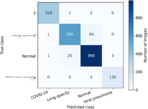
For a detailed analysis of the error distribution, the confusion matrix of the configuration with the highest diagnostic performance, ResNet50 FP32, was computed (Fig. 4.). The most difficult class for all models without exception is Lung Opacity, which is to be expected: radiologically, it is non-specific and overlaps with the other classes. The smallest class, Viral Pneumonia with only 134 test images, is by contrast recognized well, which confirms the effectiveness of class weights as a means of compensating for imbalance.

COVID-19

Lunq opacity

viral pneumonia

Fig. 4. Confusion matrix of the best configuration (ResNet50 FP32)

• 4.5.    Transfer to an Independent Dataset

• 4.6.    Localization of the Features the Model Relies On

The models trained on the primary dataset were applied to the 5,856 images of the independent Chest X-Ray Images (Pneumonia) dataset without any fine-tuning. Because the two datasets do not share a label space, the mapping between them is defined before any result is presented. The internal task has four classes and the external task two, Normal and Pneumonia, so two mapping scenarios are evaluated. In the broad scenario the internal classes COVID-19, Viral Pneumonia and Lung Opacity are all mapped to the external class Pneumonia and the internal class Normal to Normal, so that every external image receives a prediction. In the narrow scenario, the radiologically non-specific class Lung Opacity is treated as ambiguous, and images predicted into it are excluded from the comparison. Coverage in Table 8 is accordingly the share of the 5,856 external images retained by the narrow mapping; recall is the recall of the Pneumonia class and specificity the recall of the Normal class, both computed after mapping. The results under both scenarios are given in Table 8 and Fig. 5., for training seed 42, so that the ranks within the table refer to a single set of trained models.

Table 8. Results on the Independent Dataset (Training Seed 42)

Configuration	F1 Internal	F1 External, Broad	F1 External, Narrow	Coverage, %	Excluded	Recall	Specificity
ResNet50 FP32	0.9685	0.9784	0.9784	99.98	1	0.9881	0.9690
ResNet50 INT8	0.9654	0.9794	0.9794	99.98	1	0.9895	0.9684
EfficientNet-B0 FP32	0.9584	0.9635	0.9635	100.00	0	0.9864	0.9311
EfficientNet-B0 INT8	0.4542	0.4238	0.4238	99.93	4	0.9998	0.0019
MobileNetV3-Small FP32	0.9573	0.9706	0.9706	99.98	1	0.9883	0.9463
MobileNetV3-Small INT8	0.1014	0.4213	0.4170	95.51	263	0.9977	0.0000
TinyCNN FP32	0.8962	0.9212	0.9216	99.83	10	0.9775	0.8393
TinyCNN INT8	0.8888	0.9226	0.9236	99.71	17	0.9761	0.8479

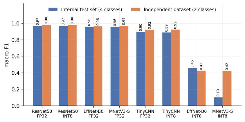
Fig. 5. Performance on the internal test set versus the independent dataset (Training Seed 42)

The values obtained on the external dataset are higher than the internal ones, yet this is not evidence of better generalization, and such an interpretation would be a methodological error: the external task is binary, Normal versus Pneumonia, whereas the internal task has four classes, and a simpler task predictably yields higher absolute values of the F1 metric. The correct scientific interpretation is that the performance of the models does not degrade on an independent sample. The key observation is that the overall ranking hierarchy of the architectures is strongly preserved across the two datasets: the rank correlation between the internal and external ordering is Kendall's т = 0.912 over the 14 configurations evaluated externally, namely the eight of Table 8 together with the six ablation variants of Section 4.7. The deviation between the two mapping scenarios defined above is minimal for every operational configuration, because the narrow mapping retains more than 99% of the external images; the conclusion is therefore not an artifact of the mapping rule. The one exception is MobileNetV3-Small INT8, whose coverage falls to 95.51%, that is, 263 of the 5,856 images, and whose specificity is 0.000; EfficientNet-B0 INT8 behaves in the same way with a specificity of 0.002. Both are further symptoms of the collapse documented in Section 4.3 rather than properties of the external dataset, and in both cases, the high recall of 0.998 is a symptom of the breakdown and not a merit.

The gradient-weighted class activation mapping (Grad-CAM) method [22] was used to interpret the decisions; 238 overlays were produced across the four architectures and the three training seeds, separated into correct and erroneous decisions. The perceptually uniform Magma color map was used instead of the widespread Jet, because rainbow maps create spurious boundaries where the gradient is smooth and are poorly legible for readers with color-vision deficiencies. The opacity of the overlay is proportional to the activation, so the anatomy remains visible.

Two observations follow, and they do not point the same way. Qualitatively, in correctly classified cases (Fig. 6, a and b) the activation is concentrated within the lung fields, and for the Lung Opacity class, it lies in the peripheral regions, which corresponds to the radiological semantics of the class; in individual erroneous cases, the activation is instead located at a corner of the frame (Fig. 6. c) or over the mediastinum (Fig. 6. d). Quantitatively, however, the center of mass of the heat map did not leave the central 20–80% band of the frame in any of the 238 overlays, for correct and erroneous decisions alike. Peripheral activation therefore occurs in individual images but is not a systematic accompaniment of error.

The discrepancy is itself the useful result because it bears on the safeguard rather than on the model. The measurement pipeline computes the center of mass of the heat map automatically and treats values outside the 20–80% band as an indication of reliance on irrelevant regions. On this sample, that criterion fired for none of the 238 overlays, including those in which a peripheral hot spot is plainly visible, because a single off-center maximum is averaged away by diffuse activation elsewhere. The center of mass is therefore too coarse a statistic to serve as the safeguard it was introduced to provide, and a criterion based on the spatial distribution of the activation, or on its overlap with a lung mask, is required instead. Establishing whether the model attends to the pathology itself needs annotation that the datasets used here do not contain.

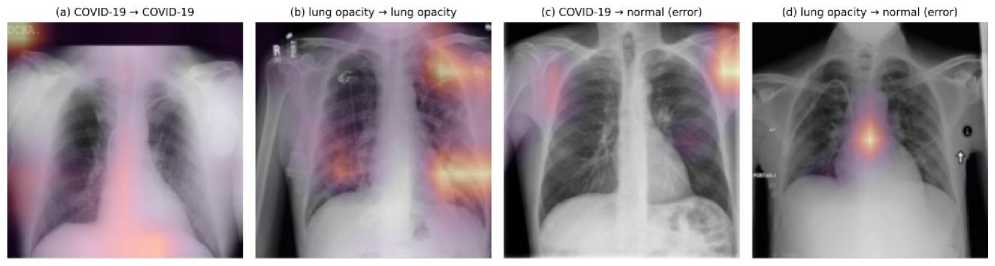
Fig. 6. Feature localization by Grad-CAM (MobileNetV3-Small FP32)

• 4.7.    Ablation of the Custom Network

5.    Practical Application of the Results 6.    Conclusions

TinyCNN was introduced above as the lower bound of the cost axis, and whether its two structural parameters are justified is examined here. Three further configurations were trained at training seed 42, each altering one parameter of the baseline network of width 32 and five blocks (Table 9). Reducing the depth from five blocks to three costs 12.9 percentage points of macro-F1, whereas halving the width to 16 channels costs 6.7, so depth is the more valuable of the two parameters. The shallow variant is, moreover, dominated outright: it is both worse than the narrow variant and 73% more expensive in computation, which justifies the choice of five blocks. Widening the network to 48 channels buys 1.2 percentage points for twice the computation, so the baseline width is a deliberate choice in favour of cheapness and not a maximum of performance, and it is described as such. Measured by performance per unit of computation, the best point of the family is not the baseline but the narrow variant, at 21.4 macro-F1 per GFLOP against 7.31, which is a sensible configuration for pre-sorting a stream of studies but not for diagnosis.

Table 9. Ablation of the Custom Network (One Parameter at a Time, Training Seed 42)

Configuration	Width	Blocks	Parameters, M	GMACs	Macro-F1	Latency, ms	Macro-F1 per GFLOPs
TinyCNN d3	32	3	0.048	0.034	0.7677	1.58	11.41
TinyCNN w16	16	5	0.036	0.019	0.8290	1.00	21.36
TinyCNN (custom)	32	5	0.135	0.061	0.8962	2.22	7.31
TinyCNN w48	48	5	0.297	0.126	0.9079	3.85	3.61

Note: The efficiency values in Table 9 are computed at training seed 42; the corresponding entry of 7.29 for TinyCNN in Table 3 is the mean over three training seeds.

The quantitative assessment of the trade-off between diagnostic accuracy and computational complexity provides a methodological basis for deploying lightweight convolutional neural networks in a production environment. The measured resource profiles make it possible to formulate differentiated deployment recommendations depending on the hardware constraints of the target infrastructure. For the typical scenario, a primary chest X-ray analysis service on CPU-only hardware without a graphics accelerator, the recommended configuration is MobileNetV3-Small FP32: a macro-F1 of 0.956 at 4.36 ms per image on a single core, 5.81 MB on disk, and 83 MB of random-access memory. EfficientNet-B0 does not displace this recommendation: the two are statistically indistinguishable in performance (p = 0,77), while EfficientNet-B0 requires 6.8 times more computation and 4.8 times more latency, so the more recent architecture buys nothing for its price. Where the model size is the stricter constraint, as on embedded and edge devices, TinyCNN INT8 is the alternative: 0.19 MB, that is, 473 times smaller than the ResNet50 FP32 baseline, and 1.23 ms per image at a macro-F1 of 0.888. The INT8 variants of MobileNetV3-Small and of EfficientNet-B0 are deliberately not recommended, since, despite the best formal resource indicators, those models are non-functional, as shown in Section 4.3. For ResNet50 and for the whole TinyCNN family, by contrast, quantization is free within statistical error and should be applied.

The resulting models and the measurement protocol form the basis of a prototype inference service implemented as an ONNX Runtime application with a microservice interface: images are processed one at a time, with a batch size of one, which matches the measurement regime, and the result card reports, in addition to the class and the confidence level, a Grad-CAM overlay and the actual resource indicators of the inference performed. Reporting latency and model size in the interface is not a decorative element but a control mechanism: it allows operating personnel to detect a degradation of performance on specific hardware without separate tooling. The general cloud architecture of such a service was considered by the authors earlier [23]. The decision of the model has the status of a recommendation and is subject to confirmation by a physician.

This work experimentally investigated the trade-off between diagnostic performance and the computational cost of neural network models for chest X-ray classification, which yielded the following results.

The computational gap was quantified. A computation performed with a single tool for 15 widely used architectures revealed a 323-fold gap in the number of operations between the heaviest architecture (VGG19) and the lightest one, whereas the published difference in accuracy on chest X-ray tasks is measured in single percentage points. The default choice of a heavy architecture has no computational justification.

The actual price of moving to a lightweight model was established. MobileNetV3-Small trails the heavy ResNet50 baseline by only 1.24 percentage points of macro-F1 (0.9557 versus 0.9681 as a mean over three training seeds; 95% confidence interval 0.84 to 1.63) while requiring 69 times fewer operations, 19.3 times lower latency on a single CPU core and a 15.4 times smaller model. The gap is about six times the standard deviation of training and is significant under both a paired t -test across seeds and a paired bootstrap over the test set. The efficiency indicator, macro-F1 per GFLOP, differs by a factor of 68, which is direct quantitative confirmation of the hypothesis of the study: the final fraction of accuracy costs a disproportionate amount of computation.

A limit of applicability of quantization was identified and documented. Post-training quantization yields a 3.91-fold compression and a 3.58-fold speed-up for ResNet50 at the cost of 0.52 percentage points of macro-F1, a loss that is not significant after correction, yet it destroys both architectures that place a Squeeze-and-Excitation block after a depthwise convolution: MobileNetV3-Small falls to a macro-F1 of 0.0887 at a ROC-AUC of 0.5615 and EfficientNet-B0 to 0.5311, in three runs out of three, and none of the eight quantization configurations tested restores operability. A controlled comparison across the four architectures exonerates both depthwise convolutions and the Hard-Swish activation and isolates the Squeeze-and-Excitation block as the cause; the number of channel-wise multiplication nodes in the exported graph separates the failing from the surviving architectures exactly and can be read off before training. Hence the engineering rule: the quantizability of a lightweight model has to be verified by measurement rather than assumed, since the risk is highest exactly where the resource gain is most desirable.

The conclusions were checked against independent data. On a dataset not used in training, the performance does not degrade and the overall ranking hierarchy of the architectures is preserved with a rank correlation of Kendall's т = 0.912, so the conclusion regarding the suitability of lightweight models is not an artifact of the primary dataset. The proposed safeguard against reliance on irrelevant features was found to be insufficient. Across 238 Grad-CAM overlays, the center of mass of the heat map never left the central 20–80% band of the frame, for erroneous decisions as much as for correct ones, even though individual erroneous overlays show activation at a corner of the frame or over the mediastinum. Peripheral activation is therefore not a systematic accompaniment of error, and the center-of-mass criterion is too coarse to detect the individual cases that do occur; a criterion based on overlap with a lung mask is the appropriate replacement.

The main contribution of this work lies in establishing a reproducible CPU resource profile for chest X-ray classification models and a verification method for the boundary of post-training quantization, rather than in proposing a new architecture. It is therefore twofold: the performance-to-resource trade-off is quantified under a single unified protocol, and a failure case of post-training quantization is documented in full together with the remediation attempts that did not resolve it. The study identifies a configuration, MobileNetV3-Small FP32, that delivers competitive diagnostic performance at low computational complexity and modest hardware requirements, and supplies the measured basis on which such a configuration can be selected for a stated resource budget. No claim of optimality is made for the custom TinyCNN network: the ablation in Section 4.7 shows that its width is a deliberate choice in favour of cheapness rather than a maximum of performance, while its depth is justified, the shallower variant being dominated outright.

The limitations of the study and the directions for further research are as follows. The split is image-level rather than patient-level, since the datasets used contain no patient identifiers, which may inflate the performance estimate. Each of the four principal architectures was trained three times, but three seeds remain a small sample: the confidence intervals of the across-seed tests are correspondingly wide, and the ablation points of Section 4.7 were trained once and carry no variance estimate. Four of the 15 costed architectures were trained, so the comparison contains no measured performance or latency for MobileNetV2, SqueezeNet 1.1, ShuffleNetV2-x1.0, or ConvNeXt-Tiny; their computational cost appears in Table 1, and extending the trained set is a direct continuation of this work. The absolute latency values were measured on specific hardware and remain hardware-dependent; for a target platform they should be re-measured under the same protocol. Of the compression methods, only quantization was implemented; pruning, knowledge distillation, and quantization-aware training are the subject of the next stage. In particular, the hypothesis that quantization-aware training rescues architectures containing Squeeze-and-Excitation blocks was not tested here, and the interpretability analysis rests on a coarse spatial statistic rather than on annotated pathology, as Section 4.6 states. The system developed is a decision support tool and not an autonomous diagnostic agent.

All the Declarations and StatementsAuthor Contributions Statement

Kateryna P. Hazdiuk – Conceptualization, Methodology, and Supervision: proposed the research idea, constructed the overall framework, and supervised the execution of the study.

Roman V. Movcheniuk – Software Implementation, Data Curation, Model Training, Validation, Formal Analysis, and Writing – Original Draft: implemented the experimental pipeline, prepared the datasets, trained and profiled the models, analyzed the results, and drafted the manuscript.

Both authors contributed to Writing – Review and Editing and have read and agreed to the published version of the manuscript.

All authors have read and agreed to the published version of the manuscript.

Conflict of Interest Statement

The authors declare no conflicts of interest.

Funding Declaration

This research received no specific grant from any funding agency in the public, commercial, or not-for-profit sectors.

Data Availability Statement

This study analysed publicly available datasets. The COVID-19 Radiography Database is available at , and the Chest X-Ray Images (Pneumonia) dataset is available at (both accessed on 24 August 2026).

Ethical Declarations

This study did not involve human participants or animals. It was performed exclusively on publicly available, deidentified chest X-ray datasets, so no ethical approval was required.

Acknowledgments

N/A

Declaration of Generative AI in Scholarly Writing

Language polishing, grammar and formatting were done with the help of AI. There was no use of a generative AI to create content, generate ideas, analyse data, generate figures, or write scientifically.

Abbreviations

The following abbreviations are used in this manuscript:

CNN - Convolutional Neural Network

CPU - Central Processing Unit

COVID-19 – Coronavirus Disease 2019

FLOP - Floating-Point Operation

FP32 - 32-bit Floating-Point Representation

GPU - Graphics Processing Unit

Grad-CAM - Gradient-weighted Class Activation Mapping

INT8 - 8-bit Integer Representation

MAC - Multiply-Accumulate Operation

ONNX - Open Neural Network Exchange

PTQ - Post-Training Quantization

QAT - Quantization-Aware Training

QDQ - Quantize-Dequantize Format

RAM - Random-Access Memory

ROC-AUC - Area Under the Receiver Operating Characteristic Curve

Appendix A/B/C…, with appendix title

N/A