Customer Credit Risk Assessment using Artificial Neural Networks

Published Online March 2016 in MECS

Since most of financial bank resources are used as facilities and the main revenue of banks is provided by this section as well, granting credit is considered as the most important consumption of financial bank resources. Because these resources are limited, banks should try to allocate these resources to develop the manufacturing and service sections with the aim of gaining more profit appropriately. In banking system, creating a customer credit risk system that can evaluate applicant’s repayment ability before granting it to them, is very important. Now there are many models and different ways to classify bank applicants that each of them is based on a particular pattern and their aim is to classify applicants into two classes; good applicants who are more likely to repay facilities and bad applicants, whose possibility of facility repayment is low. Banks as the main part of the financial system have always faced various risks. Credit risk is the most important and will cause financial problems for banks then its assessment needs advanced modelling techniques. A considerable volume of unpaid bank facilities indicates a lack of both appropriate models of credit risk assessment and risk management system in banking systems. In recent years, delayed claims are an issue that has caused a shortage of financial bank resources and has damaged to the bank. By rapid growth of banking industry, validation models are used widely to evaluate whether to grant credit to applicants or not. Some of the benefits of validation models include: 1. Reduce the cost of credit analysis 2. Immediate decisions on customer validation 3. Guarantee credits and eliminate probable risks [1, 2]. By information analysis of bank customers using data mining process, we can assess loan applicants and classify them into good or bad applicant based on intelligent systems without personal judgments [3]. In general, ANNs which are useful technique in data mining process, and as an accurate tool for credit risk assessment, has been shown to be effective over the past decade. The capability of ANNs in such applications is due to the availability of training data and the way the network operates, include: network structure and learning algorithms and etc. This is more evident when using MLP networks based on the BP learning algorithm [4]. Gradient Descent, Conjugate, One-step, Gradient Descent, BFGS Quasi-newton, Resilient Secant and LM are all different types of the BP learning algorithm [5, 6].

Therefore, in this paper six different MLP models were developed and compared to each other based on these BP learning algorithms.

There are many researches and applications in various areas of classification to identify bank applicants. In 1930, Fisher and Durand created initial validation models. Lyn in 2000 did a thorough study on probation and validation. Yu et al. in 2009, proposed a novel intelligent-agentbased fuzzy group decision making (GDM) model as an effective multi criteria decision analysis (MCDA) tool for credit risk assessment. They evaluated a simple numerical example with three real credit datasets of United Kingdom, Japan and Germany. The results clearly showed that the proposed fuzzy model GDM outperforms other comparable models [7]. Hsieh and Hung in 2010, by using ensemble classification methods, neural networks and support vector machine proposed a classification system for bank applicants [8]. Chuang and Huang in 2011 proposed a two-stage method; in the first stage a neural network was used to classify an applicant as accepted or rejected and in second stage in order to identify rejected applicants who should have been accepted, a case-based reasoning was used [9]. Akkoc in 2012, proposed a three stage hybrid Adaptive Neuro Fuzzy Inference System model (ANFIS) for credit scoring, which is based on statistical techniques and Neuro Fuzzy. He compared it with conventional and commonly utilized models. Results demonstrated that the proposed model consistently performs better than the Linear Discriminant Analysis (LDA), LR Analysis, and Artificial Neural Network (ANN) approaches, in terms of average correct classification rate and estimated misclassification cost [10]. Jochen et al. in 2013 applied machine learning methods and an optimized LR to a large dataset of complete payment histories of short-termed instalment facilities and specified prediction of the probability in random forests, probability estimation and classification. They showed that random forests outperform optimized LR, k-nearest neighbours and bagged k-nearest neighbours [11].

Following this introductory section, the rest of the paper is organized as follows: In section 2 classification methods such as ANN, Decision Tree and LR are defined respectively. Section 3 is allocated to the methodology of this paper. Then model performance assessment criteria which are Accuracy, MSE, Type Ι error, Type ΙΙ error and AUC are defined in related subsections. The simulation results of comparing the proposed model with two other models are stated in section 4 and finally section 5 is allocated to the conclusion of this study.

• II.    Classification Methods

In the credit risk assessment literature, many classified techniques including traditional statistical techniques, such as LDA, LR, quadratic discriminant analysis and non-parametric models, such as k-nearest neighbour, Decision Trees and ANN have been proposed. In the following three classifiers, ANN, Decision Tree and LR will be discussed

• A.    Artificial Neural Network

Among different non-parametric models, ANN has developed recently in different sciences particularly in machine learning. This technique can be used both in discovering and extracting knowledge from database and also for creating prediction models. Neural network is used to model the relationships between inputs and outputs and to find the patterns in the dataset. Training neural network is a challenging problem we encounter while working with them. ANN is an adaptive system that changes its structure during the learning stage. Focusing too much on training data is likely the main problem in neural network training process [12]. Proper selection of number of neurons in the hidden layer and number of layers prevent excessive concentration on training data and thereby lead to fix this problem. Both learning ability of ANN and the Accuracy of predicted output are determined by the number of neurons in the hidden layer. If the number of neurons in the hidden layer is too low, complex relationships between inputs and outputs of the neural network cannot be found and convergence of neural network training may be in trouble. On the other hand, if this number is too much, the training process will take longer and can cause harm generalizability of neural networks [13].

The most common neural network model is the MLP, which is a feed-forward neural network with three layers: input and an output layers with one or more hidden layers between them. Generally, BP algorithm is used to train the MLP neural network. BP is one of the most popular learning algorithms based on reducing error and is formed in a supervised manner and generates a response based on random weights. In an iterative process the error rate between network output and actual values (target) decreases according to changing weights. This procedure starts from output node and continues backwards computation.

• B.    Logistic Regression

LR is a special case of generalized linear models which is used as a function of independent variables for predicting the probability of a binary (nominal or ordinal) variable that the probability value changes between 0 and 1. Since the outcome variable in LR is divided into two parts (0 and 1), it leads to discern a LR model from a linear regression model which allows the dependent variable to take values greater than 1 or less than 0. LR models have been widely used in credit assessment applications, due to their simplicity to implement. In this paper, the dependent variable is considered as a binary variable, in which ‘0’ refers to good applicants and ‘1’ allocates to bad applicants.

• C.    Decision Tree

Decision Tree is a technique that shows knowledge in large amounts of data. Although there are some limitations, Decision Tree is one of the most popular techniques, as a powerful and flexible tool in classification and prediction and also an appropriate tool for knowledge discovery. One of these limitations is that they are unstable; it means that small changes in the data samples may cause big changes in classifying them. The structure of Decision Tree is similar to the structure of a flowchart in which each intermediate node represents a test on one or more attributes. Each branch shows the test output and each leaf node contains a class label. Decision Tree can generate intelligible rules. Even in a large or complicated tree we can easily pass through a direction that it makes the interpretation of classification or prediction to be relatively easy. Decision Tree explains its predictions in rule sets, while in neural networks because it is considered as a black-box technique, the final prediction is shown and its condition is left hidden in the network, so this is the counterpoint of these two methods. Decision Tree algorithm known as ID3 was developed by Quinlan in the late 70s and early 80s [14, 15]. After ID3, C4.5 was presented which have two advantages compared to ID3, having more than two children for each node and using pruning techniques. In this paper, among different Decision Tree algorithms, C4.5 was considered to compare with the proposed ANN model.

• III.    Methodology

In this study, we use the UCI machine learning database, one of the 100 reliable databases, which has the most references in scientific papers available via The German, Australian and Japanese datasets are the three credit datasets used in this study to compare the performance of presented model with other classifiers. These datasets have been used for credit scoring and credit assessment systems successfully in previous works [7, 16, 17 and 18]. Table 1 shows a summary of the main features of these credit datasets.

Table 1. Some Details of Datasets used in Study

No.	Dataset	No. of Attributes	No. of Good Instances	No. of Bad
1	German	21	700	300
2	Japanese	15	296	357
3	Australian	14	307	383

In data normalization process, the input data are normalized between 0 and 1. This is performed by finding the maximum number in each column (feature) for all instances and dividing the rest of the entries in each column to its maximum value. To assess the reliability and validity of the model, the dataset is randomly divided into three sets of training, validation and testing data. In this study, 60% of data considered as training data for building the model, 10% as validation data and 30% were considered for testing the model.

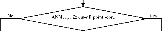
In this study, in order to find the best ANN, we use an MLP neural network (consists of three layers; input, output and one hidden layer) with six BP learning algorithms shown in Table 2. The output layer consists of one neuron that produces a binary output, ‘0’ for good applicant and ‘1’ for bad applicant. At first, a cut-off point score 0.5 is considered to distinguish between these two groups. In a single cut ‐ off point, the applicant’s total score is compared with a cut‐off point score. If this score is greater than the cut‐off point score, applicant’s credit status will be bad, otherwise it will be good.

Table 2. Different BP Learning Algorithms

No	Abbreviation	Learning Method Description
1	LM	Levenberg–Marquardt
2	GD	Gradient descent
3	CGD	Conjugate gradient descent
4	R	Resilient
5	BFGS	BFGS quasi-Newton
6	OS	One-step secant

The nonlinearity power of MLP appears, when all MLP neurons use a nonlinear activation function to calculate their outputs. The whole MLP will become as a simple linear regression machine, if we use a linear activation function. In this paper, we have used two most common activation functions from logistic family, the Sigmoid function and the Hyperbolic Tangent function which are the most greatly used in MLP implementation.Another factor which should be considered in constructing an ANN is the number of neurons presented in the hidden layer. Each of six networks runs and trains for different numbers of neurons from 10 up to 40 within their hidden layer. Training process performs 10 times for each number of these neurons as well. MSE is a criterion to specify optimum number of neurons in the hidden layer calculated by equation (1). The mean value of MSE for performing training process (10 times), is considered as the MSE main value for each number of neurons in the hidden layer. MSE is a common criterion to obtain the best estimator. By using this criterion, the estimator with lowest MSE is selected and we aim to minimize this value during the training process. MSE is actually one of several ways that indicates the difference between the predicted and real value by estimator.

- ¹ V , в = у —у, MSE = — / е

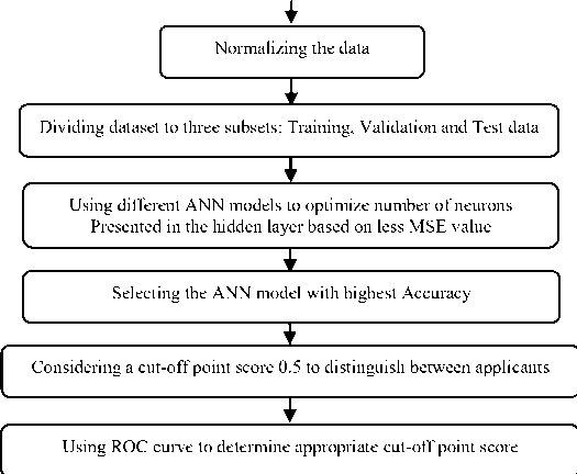
Where, (e) presents the error rate and shows the difference between predicted (y) and actual value (y). Also, to assess the performance of ANNs, their Accuracy is evaluated based on the optimum number of neurons (obtained in prior step) in the hidden layer. Like MSE, by 10 times performing the training process, the mean value of Accuracy was considered. In the following, the ROC curve was used to specify the appropriate cut-off point score which is an important factor in customer credit risk assessment systems in order to decrease the number of bad applicants that wrongly recognized as good applicants. Fig. 1 shows a flowchart of implementation of the proposed model that is constructed by three-layer perceptron neural network with different numbers of neurons and six types of learning algorithms which aim to detect the best neural network for bank customer classification.

Definition of inputs and output

Labeling results to Good applicants

Labeling results to Bad applicants

Fig.1. Methodology flowchart

Model Performance Assessment Criteria

The performance assessment criteria used in this study include Accuracy, MSE, Type I and Type II errors. These standard criteria in the field of credit risk assessment are used in many previous studies [1, 19 and 20]. Each criterion has its merits and limitations. In this study a combination of these measures is preferred to use rather than a single measure to evaluate the performance of enterprise credit risk assessment models. The MSE was obtained in section 3 in this study. Most of the assessment criteria can be easily obtained from confusion matrix that is a useful tool for analyzing how classification method works in data recognition or observation of different classes. For a two-class problem, most of performance assessment criteria can be easily derived from a 2*2 confusion matrix as that given in Table 3. Each element in this matrix represents the number of correct or incorrect predictions of applicant’s positions in categories. The ideal state of confusion matrix to have high Accuracy in classification is when the matrix is created diagonal form, i.e. most of data are located on the main diagonal of the matrix and the rest of

the matrix values are zero or close to zero.

Table 3. Confusion Matrix

Real class

Test output

Bad applicant

Bad applicant             TP

Good applicant           FN

Good applicant

FP

TN

Where; TP (True Positive): the class of bad applicant, correctly diagnosed as bad; FP (False Positive): the class of good applicant, wrongly diagnosed as bad; FN (False Negative): the class of bad applicant, wrongly diagnosed as good; TN (True Negative): the class of good applicant, correctly diagnosed as good.

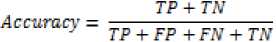
1). Classification Accuracy

Classification Accuracy indicates the proportion of the correctly classified cases (both good and bad applicants) on a particular dataset. The classification Accuracy is considered as success ratio of a model i.e. the ratio of

True Positive and True Negative (Which are correctly predicted) on specific datasets. It can be defined as equation (2):

Type II error =

FN + TP

However, the Accuracy ignores the different cost of both error types (bad applicants being predicted as good, or vice versa). This is the reason why it becomes especially interesting to measure the error on each individual class by using the Type I and Type II errors.

• 2) . Type I and Type II error

In financial institutions, the cost that Type II error rate imposes to the system is too high. Hence, we are always looking for a model that in addition to high Accuracy has lower Type II error rate. Type Ι and Type ΙΙ error criteria are often very different. Generally, misclassification costs associated with the Type ΙΙ error is greater than Type I error rate. West expressed that misclassification cost is associated with the Type Ι and Type ΙΙ error as 1:5 [21]. In addition, because Type ΙΙ error causes bank losses, we should pay more attention to the Type ΙΙ error.

Type I error: is the rate of good applicants being predicted as bad. Type I error is given by equation (3),

_              FP

Type I error = ——— ^,r         FP + TN

Type II error: is the rate of bad applicants being classified as good. So, the misclassified bad applicants will become as a defaulter. Type II error is given by equation (4),

• 3) . Area under Curve

Receiver Operator Characteristic curves (ROC) are a graphical representation of the trade-off between False Positive rate on the x-axis against True Positive rate on the y-axis for all cut-off point scores. In order to compare the ROC curves of different classifiers, the Area under the ROC curve (AUC) must be computed. This is a measure of the discrimination power of a classifier regardless of class distribution or misclassification cost [22]. By choosing the cut-off point score, the analyst can control the probability of the correct recognition of the Positive and Negative outcomes. When reducing the cutoff point score, the False Positive outcome increases. Although the test is highly sensitive, it’s not very particular and conversely, by maximizing the cut-off point score, the False Negative outcomes will increase. Although the test is highly particular, but it is not very sensitive. Sensitivity is defined as the probability that the classification model will produce a positive result for a client who is a defaulter, and Specificity is defined as the probability that a classification model will produce a negative result for a client who is not a defaulter.

• IV.    Results and Discussions

At first, the optimum number of neurons in the hidden layer specified according to the minimum value of MSE on test data.

Table 4. The Performance of ANN Models with six BP Learning Algorithms

Dataset	No.	Learning Method	Optimum No. of neurons in hidden layer	MSE	Accuracy
German	1	LM	22	0.1821	76.80%
	2	GD	37	0.2383	68.26%
	3	CGD	19	0.1899	71.92%
	4	R	17	0.1662	74.84%
	5	BFGS	18	0.1656	75.40%
	6	OS	11	0.1697	74.80%
Japanese	1	LM	16	0.1069	88.49%
	2	GD	35	0.2210	76.87%
	3	CGD	13	0.1048	84.21%
	4	R	16	0.1079	85.88%
	5	BFGS	16	0.0947	86.01%
	6	OS	17	0.0994	85.75%
Australian	1	LM	22	0.1118	88.31%
	2	GD	40	0.2028	78.11%
	3	CGD	14	0.1022	85.98%
	4	R	35	0.1017	86.%26
	5	BFGS	11	0.0996	86.71%
	6	OS	19	0.1034	85.88%

The performance of six different BP learning algorithms were evaluated based on MSE and Accuracy. The obtained results of implementation of the MLPNN models with these learning algorithms are listed in detail in Table 4 which shows that the preferred ANNs, are the ones using LM algorithm. For German, Japanese and for Australian dataset, the MSE achieved are 0.1821, 0.1069 and 0.1118 respectively. For each dataset, the highest Accuracy value of all models is highlighted in bold face. In order to simulate the considered MLP neural networks,

MATLAB version R2012a software was used.

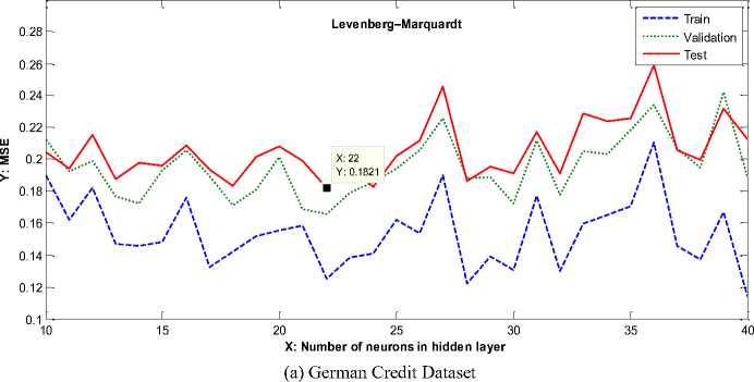
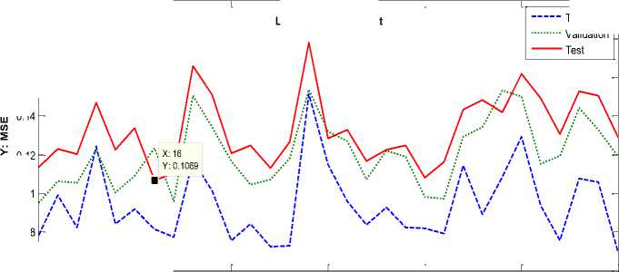
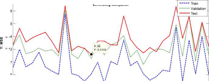
As can be observed, LM Back-Propagation (LMBP) outperforms than other learning algorithms. Therefore, in this study LMBP is used as the proposed algorithm in training the MLP neural network. The MSE changes to the number of neurons within the hidden layer per testing, validation and training data with LMBP, are shown in Fig. 2(a)-(c) for German, Japanese and Australian datasets respectively when minimum MSE has been occurred.

Train

Validation

0.2

Levenberg–Marquardt

0.18

0.16

0.12

0.1

0.08

0.06 10

X: Number of neurons in hidden layer

(b) Japanese Credit Dataset

0.2

Levenberg-Marquardt

0.18

0.16

0.12

0.1

0.08

X: Number of neurons in hidden layer

(c) Australian Credit Dataset

0.06

Fig.2. MSE Changes to the Number of Neurons within the Hidden Layer per Testing, Validation and Training Data with LMBP Learning Algorithm for Each Dataset

Table 5 shows the results of our proposed ANN model compared with C4.5 decision tree and LR models. These models are compared based on Accuracy, MSE, Type Ι error, Type ΙΙ error and AUC. It is important to note that in the proposed model, at first the cut-off point score is considered as 0.5.

As can be seen from Table 5, the results showed that the MLPNN model outperforms LR and C4.5. MLPNN model obtained the highest Accuracy, lowest Type I and Type ΙΙ errors and lowest MSE when all methods were implemented. This model is highlighted in bold face in each dataset. We also observe that AUC of the MLPNN model is larger than other models, this difference indicates that the MLPNN has a greater discrimination power. However, the important disadvantages of an MLP model include its black-box nature which represents the resulting model with difficulty to interpret and also shows its long training process in designing the topology of the optimal network. Despite these disadvantages of MLP models, due to the high Accuracy and lower Type ΙΙ error rate of the model, employing this model can be very effective in customer assessment.

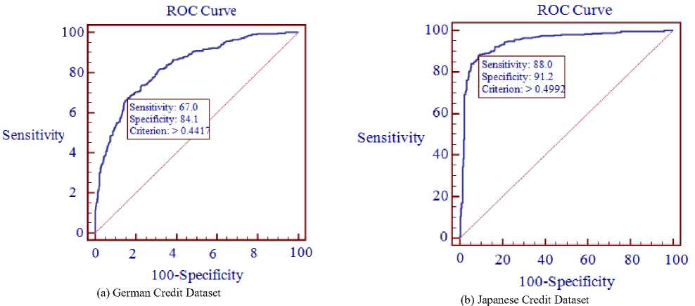
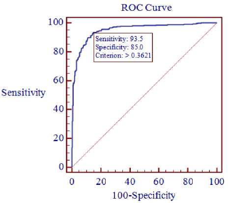
The AUC value ranges from 0.5 to 1. The larger the AUC value, the more accurate the credit scoring model is. In case of a perfect model, the AUC will equal to 1, while an area of 0.5 reflects a random model. When the AUC value is greater than 0.7, it means the model has a good discriminating capacity [23]. The ROC curves obtained by MLPNN are shown in Fig. 3(a)-(c) for German, Japanese and Australian datasets respectively.

Table 5. Implementation Results and Comparison of Assessment Criteria

Dataset	No.	Model	Accuracy	MSE	Confusion Matrix		Type Ι error	Type ΙΙ error	AUC
German	1	MLPNN	78.40%	0.1593	166 134	82 618	11.71%	44.66%	0.829
	2	LR	75.90%	0.3127	150 150	91 609	13%	50%	0.792
	3	C4.5	70.70%	0.3459	117 183	110 590	15.71%	61%	0.641
Japanese	1	MLPNN	89.12%	0.1117	312 45	26 270	8.73%	12.60%	0.944
	2	LR	85.75%	0.2139	292 65	28 268	9.45%	18.20%	0.918
	3	C4.5	85.29%	0.2021	310 47	49 247	16.55%	13.16%	0.887
Australian	1	MLPNN	88.40%	0.0946	335 48	32 275	10.42%	12.53%	0.950
	2	LR	85.21%	0.2150	317 66	36 271	11.72%	17.23%	0.914
					335	48
	3	C4.5	86.08%	0.1938	48	259	15.63%	12.53%	0.867

(c) Australian Credit Dataset

Fig.3. MLPNN ROC curves for each dataset

As mentioned in the prior section, because the Type ΙΙ error causes bank losses, we focus on this type. By setting an appropriate cut-off point score, there will be a proper trade-off between model abilities to identify good and bad applicants. However, a cut-off point will be selected that has the lowest overall misclassification. Table 6 shows the performance of the proposed model with respect to the appropriate cut-off point score obtained from the ROC curve for each of credit datasets.

The results obtained from Table 6 indicate that by reducing the cut-off point score, the Type ΙΙ error value has been decreased by 11.66%, 0.56% and 6.01% for German, Japanese and Australian datasets respectively. It is important that determination of the most appropriate cut-off point depends on the purpose of validation. Since in the bank customer credit risk assessment systems, detection of bad applicants has been more important, by setting a lower cut-off point, the ability of model to detect the bad applicant increases.

Table 6. Implementation Results by Appropriate Cut-off Point Score

Dataset	Model	Cut-off point	Accuracy	MSE	Confusion matrix		Type Ι error	Type ΙΙ error
					201	111
German	MLPNN	0.4417	79%	0.1593	99	589	15.85%	33%
Japanese	MLPNN	0.4992	89.28%	0.1117	314	27	9.12%	12.04%
					43	269
Australian	MLPNN	0.3621	89.71%	0.0946	358	46	14.98%	6.52%
					25	261

• V.    Conclusions and Future Works

In this paper, we presented a MLP neural network (MLPNN) for customer credit risk assessment. Neural networks have high power and an ability in accurate estimation of nonlinear relationships, although they have some limitations. One of these Limitations is performing as a black box, also the training of these networks is critical. The MLPNN was used with six BP learning algorithms and different numbers of neurons from 10 up to 40 within their hidden layer. The optimum number of neurons in the hidden layer specified according to the minimum value of MSE on test data. Among all BP learning algorithms, LM achieved the best performance. Hence, LMBP learning algorithm was used in training the MLP neural network. In order to implement our proposed model and compare the performance of that with other classifiers, we used German, Japanese and Australian credit datasets. Also a comparison between the proposed model, LR and C4.5 decision tree models was done. Accuracy, MSE, Type Ι error, Type ΙΙ error and AUC are the criteria that were selected for the evaluation model and in order to decide upon an ideal model. ROC curves were used to determine the appropriate cut-off point score in order to increase the Type ΙΙ error which is the most important criteria in credit risk assessment. The result showed that the proposed model was very effective and leads a system to be able to correctly classify the inputs with high Accuracy and outperforms the other two models in predicting customer credit risk.