Data Cleaning In Data Warehouse: A Survey of Data Pre-processing Techniques and Tools

Published Online March 2017 in MECS

• I.    Introduction

  Today’s real world databases are gigantic in size, and therefore, highly inclined to noisy, missing and capricious data that is inconsistent and brings about low-quality data and consequently cannot be utilized for data mining. Business Intelligence based decisions are based on clean data (Debbarma, Nath et al. 2013). So before storage, data needs to be preprocessed, in order to improve productivity of ETL (Extraction, Transformation, and Loading) process. Fig.1 provides the complete illustration of ETL process, data cleaning is performed in data staging area.

Data Cleaning routines shall be applied to “clean” the data by filling in missing attributes and values, smoothing and leveling noisy data, identifying and removing outliers, determining and settling inconsistencies (Jony, Mohammed et al. 2015). And this data cleaning is performed in data staging area before Transformation stage of ETL. Although programmed techniques are available for data cleaning, but are not fully robust. ETL tools, however, with proprietary API’s allow the user to specify the cleaning functionalities. But still there is a need to limit the manual effort (Cravero and Sepúlveda 2012).

Recent literature studies have revealed that dirty and erroneous data inflicted daunting cost upon the business organizations, also leading to degradation in performance. Thus to clean data, various tools have been introduced to resolve record-matching in case of de-duplication and then data-repairing and merging issues (Fan, Ma et al. 2014).

For cleaning data, there shall be clear disparity between instance-related and schema-related problems that exist in (single, multiple) data sources. If and once, these problems are identified it will definitely help to achieve the business objectives.

Pitfall of this effort, needed for data cleaning during extraction and integration, is increasing response times but is necessary to achieve query-optimization and data quality (Misra, Saha et al. 2013).Thus, data cleaning is an on-going process that requires awareness of underlying fundamental principles that are subjected to performance improvement (Chaturvedi, Faruquie et al. 2015). This paper provides an overview of the data cleaning problems and a study of their solution. Next section presents review of related previous work done during the ETL process to clean the data. Section 3 lays an emphasis on data pre-processing techniques, and problems and their solutions as well. Section 4 presents missing values and ways to handle it and then algorithms for missing values are evaluated with the help of some tools. Section 5 presents materialized views for query optimization to improve the performance. Section 6 presents the evaluation attributes to analyze the performance improvement. Section 7 presents the available frameworks related to data cleaning of heterogeneous sources. Section 8 presents summarized facts of commercial tools available for data cleaning. Finally, Section 9 concluded the results and anticipated future directions.

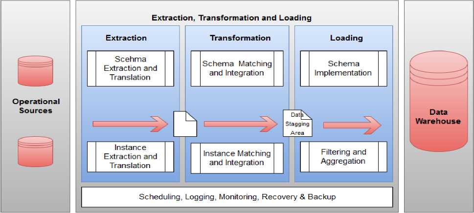
Fig.1. Overview of ETL Process

• II.    Related Work Review

  Many authors have proposed algorithms for data cleaning in past decade (Soma & Nedu et al. 201l) discussed that data cleaning is the most critical stage of data mining to remove inconsistency and noise in the data. Most common inconsistency type is missing data. Missing values cause problems like loss of precision due to less data, computational issues due to holes in dataset and bias due to distortion of the data distribution. To solve the missing data issue, algorithms have been proposed in the past. These algorithms fill the missing values and smooth out the noise. Three of those implemented algorithms are Constant Substitution, Mean attribute value substitution and Random attribute value substitution method (Somasundaram and Nedunchezhian 2011). These methods have been tested on the standard WDBC dataset and their performance has been compared on the basis of defined evaluation attributes. Results have been shown in tabular and graphical form. Results conclude that 1^st Approach of constant substitution method loses too much useful information, so gives poor results as compared to other two methods. 2^nd approach of mean attribute value substitution method is time consuming & expensive, but gives best results for missing values problem. 3^rd approach of random attribute value substitution method causes distortion in data distributions by assuming that all missing values are with the same value, however this method still manages to provide comparable results (Somasundaram and Nedunchezhian 2011). Weak point of these techniques is the need of strong model assumptions. To satisfy the missing data issue, only solution is good design of data warehouse but good analysis can somehow help in solving this problem too.

Another approach to increase efficiency of data warehouse is creation of Materialized Views (MVs), which improves data warehouse performance by preprocessing and avoiding complex resource intensive calculations (Saqib, Arshad et al. 2012).Materialized views are pre-calculated results of more frequently used queries by the users, which save time of computation on run-time of querying (Mitschke, Erdweg et al. 2014). Materialized views can generate child views automatically which are pre-computed results to next level queries. These views are created by very few input parameters, reducing the user dependent activities. The comparison of complex queries vs. time series for base relation has been provided which support this concept. Time and complexity analysis has been calculated but cost analysis is needed to be measured too, for successful implementation in future. Automatic creation of child materialized view is a complex task. In future, data warehouse needs modification for selection of numeric and string attributes for exploitation to create new MVs. Attributes comprised of multimedia data had not been catered yet. Finding balanced number of MVs with high access frequency and removing remaining MVs, needs decision too as an improvement of this concept (Saqib, Arshad et al. 2012). As advancement, business intelligence has been merged with data warehouse. Impact of erroneous data and its cost has been discussed. Evaluation attributes for data quality and performance of data warehouse have been proposed. Evaluated attributes are: Completeness, Consistency, Validity, Integrity, Conformity and Accuracy (Wibowo 2015). Issues which hinder data quality and performance have been identified in each phase of Data Warehousing Process i.e. ETL (Extraction, Transformation and Loading). In Extraction level, data quality issues are mostly because of heterogeneous data sources, imperfect schema level or instance data, insufficient source data analysis and undocumented alterations. In transformation phase, data quality issues arise because of unhandled null values, inaccurate conditional statements and insufficient source data analysis. In final loading phase, data quality issues are due to lack of periodic refreshment, wrong mapping, lack of error reporting and inappropriate handling of rerun strategies during ETL. In schema design phase data quality issues like incomplete or wrong requirement analysis, late arrival of dimensions, late identification of slowly changing dimensions or multi-valued dimensions can also cause problems. Data profiling has been proposed as counter measure. Appropriate example and statistics have been used for support of their statements. For improvement, more effective profiling, better physical design and query optimization is required to build an optimized data warehouse system (Debbarma, Nath et al. 2013).

Previous surveys have presented different approaches, for data cleaning, but those approaches have their drawbacks and still unable to resolve all the data cleaning issues completely. These drawbacks need to be studied further for their best solution. Next section discusses existing data cleaning problems which require preprocessing for improvement in data quality of data warehouse.

• III.    Data Pre-processing in Data Warehouse

  It has been clearly specified that the cost of erroneous data (undocumented alterations, Imperfect Schema Definitions, Insufficient source data analysis, Unhandled null values in ETL process) on data warehouse is leading to performance degradation (Debbarma, Nath et al. 2013),

so Data Pre-processing is required to make the system’s performance better. Different kinds of pre-processing are required for different types of data. Main pre-processing types have been discussed below.

• A.    Types of Data Pre-processing

Recent studies indicate that Data Pre-Processing is of two types:

Classical Preprocessing: Classical pre-processing can be further sub-divided into following phases:

• •   Data Fusion Phase

• •   Data Cleaning Phase

• •   Data Structuration Phase

  Advanced Preprocessing: Advanced Pre-processing includes Data Summarization Phase only. Data Cleaning is an important phase that deals with all the problems related to “clean” data, and it will prepare the data for actual analysis (Jony, Mohammed et al. 2015). Data cleaning problems, requiring pre-processing have been discussed ahead.

• B.    Data Cleaning Problems

  Hitches and complications in data cleaning process are closely related to each other and should be treated in homogeneous way. Data Cleaning problems are categorized (Rahm and Do 2000) as follows:

Single-Source Problems: Single-source problems are further sub-divided into following levels:

• •    Schema Level: It lacks integrity constraints and schema is poorly designed. E.g. uniqueness property is not kept in mind and Referential Integrity rule is violated.

• •    Instance Level: It involves mainly typo- errors e.g. misspelled words, redundant values and duplications, contradictory values etc.

Multi-Source Problems: Multi-source problems are further sub-divided into following levels:

• •    Schema Level: It involves heterogeneous data models and schema designs e.g. Structural type conflicts etc.

• •    Instance Level: It involves overlapping issues, inconsistent data e.g. inconsistent aggregation, timing etc.

These problems shall be clearly differentiated (Rahm and Do 2000); if and once these are clearly spotted then there exclusion will be somewhat easier. Data Cleaning prepares the data files for analysis and is helpful in Knowledge Discovery (Wibowo 2015). If data even now encompasses dirtiness and impurities, it cannot be utilized for precise decision making (Dixit and Gwal 2014). Because Data Analysis is comprised of two-step: Firstly, Pre-Processing (Jony, Mohammed et al. 2015) and secondly Actual Processing. Once, this is preprocessed than actual processing can be performed on it and the focus of pre-processing is to improve the quality of data and eventually performance will be optimized (Jony, Mohammed et al. 2015). Data warehouse is intended to deliver Business Intelligence solutions as well as reporting (Rahman 2016). Following are the approaches presented to solve data cleaning problems.

• C.    Data Cleaning Approaches

  Data Cleaning is a gradual process that is passed through several phases like Data Analysis, Definition Data Transformation and Data Mapping Rules, Transformation, Verification, Backflow Data Analysis (Christen 2012).

Solution to Data Cleaning Problems: Most important solutions for Data Cleaning are “Record- Matching” and” Data-Repairing” methods. Matching techniques identify the similar real world objects that are presented in tuple, and repairing techniques make the database consistent and reliable by correcting the inaccuracies (Fan, Ma et al. 2014). And these two techniques are applied on the dirty data to make it “clean” followed by certain constraints (Wibowo 2015).

Research activities still need data quality improvements, with regard to data cleaning approaches because more efficient the approach will be, better the results will be. And this needs effective profiling and improvement in physical design. And this will certainly help to build an economical decision support system. Preprocessing used for missing values is most important stage in Data warehouse, so has been discussed in detail below.

• IV.    Data Pre-processing of Missing Values in Data Warehouse

  Traditional operational systems are disposed to dirty data, as they contain missing values, hence, cannot be utilized for decision making (Saqib, Arshad et al. 2012).There are following three techniques for preprocessing of missing values.

• •   Constant Substitution

• •   Mean Attribute Value Substitution

• •    Random Attribute Substitution

The above mentioned techniques of pre-processing are discussed below in detail.

• A.    Missing Data

  There may be missing attribute values in the training data sets that could not be recorded appropriately, at some point or might be ignored intentionally, due to confidentiality purposes in data collection or objects that are yet to be classified can also suffer with missing attribute values. Missing data problems are not specific to particular cases, missing attribute values are more probably written as unknown, NULL, or missing etc. A straightforward approach abandons those instances with Missing values (Somasundaram and Nedunchezhian 2011). Identification of missing values is actually a difficult task and the problems initiated by missing data are as follows:

• •    Precision loss as a result of limited data by simply discarding incomplete data instances

• •    Computational and Technical problems

• •    Misrepresentation of data

Thomas Lumley proposed following two solutions for the missing values:

• •    For missing values, compute probability weight age and use in summaries.

• •    Use implicit or explicit suggestions, related to specific data during model distribution.

More solutions for missing data handling are discussed below.

• B.    Handling of Missing data

Several data mining approaches exist to handle missing values, and depend upon the sphere of problem.

• •    Ignore the tuple in record: This approach is recommended when many attribute values are

missing in data not just one. But this approach yields low performance, if the fraction of such rows is higher. E.g. consider a database of students (name, father name, residence, city, and blood group) to predict admission rate in particular city. In this situation, missing data in blood group column can simply be ignored.

• •    Use global Constant: Decide a specific constant e.g. NULL, N/A, or hyphen etc. This is useful when filling of attribute value does not make sense. E.g. in students database, if attribute values in the “city” column are not specified, then filling up of these values is not appropriate as compared to usage of global constant.

• •    Use of attribute mean: In this method missing values are replaced with median or mean and fill them with most suitable value. Mean will be most suitable in case of discrete values. E.g. Average salary in Pakistan can be replaced by 3 lacks or according to mean.

• •    Use Data Mining algorithm: Predict values by using data mining tools and then utilize them. In market, regression based tools are available which produce K-Mean / Median etc. Also clustering techniques can be applied to make cluster of rows in order to compute aggregation functions or mean values. And to compute similarities between clusters Rand Index Measure is helpful (Somasundaram and Nedunchezhian 2011).

Some algorithms, developed for the computation of missing values, have been discussed below.

• C.    Algorithms for computation of Missing Values

  Three algorithms have been presented below, that compute missing values and their attributes (M) in dataset (D) (Somasundaram and Nedunchezhian 2011).

• •    Replacing missing values with constant numeric value: If the data contain non- numeric attributes then their computation becomes difficult, so in order to avoid complexity, an algorithm has been presented that replaces non-numeric attributes (unknown, minus infinity) with numeric attributes (0 or 1 or else) depending upon size of data to make computations easier.

Pseudo code:

For r=1 to N

For c = 1 to M

If D(r, c) is not a Number (is a missing value), then

Substitute zero to D(r, c)

• •    Replacing missing values with attribute mean:

All the data rows are removed which contain missing values in dataset D , and providing missing value “d with total records n”.

Pseudo code:

For c = 1 to M

Find mean value “Am” of all the attributes of the column “c”

Am(c) = (sum of all the elements of column c of d)/n

For r=1 to N

For c = 1 to M

If D (N, M) is not a Number (missing value), then Substitute Am(c) to D (N, M)

• •    Filling missing values with random attribute values:  Missing values are determined by

considering minimum and maximum values in dataset D .

Pseudo code:

For c = 1 to M

Find mean value “Am” of all the attributes of the column “c”

Min(c) = (min of all the values of column c) Max(c) = (max of all the values of column c) For r=1 to N

For c = 1 to M

If D (N, M) is not a Number (missing value), then Substitute a random value between Min(c) and Max(c) to D (N, M)

Missing values are crudely categorized into parametric (linear regression) and non- parametric (Kernel-based regression, Nearest Neighbor Method) values as well. Comparatively the parametric computation of missing values provides best and optimum results, if parameters are specified by users correctly. Non- parametric is excellent as it apprehend the structure of miss-specified dataset and provides alternatives to be replaced. Also when conditional and target attributes are not known then non-parametric technique is best, providing finest results. On the other hand, parametric (statistics based methods) methods of linear regression are not reasonable in solving problems of missing values.

Other algorithms for computing missing values include genetic algorithm, fuzzy similarity matrix. These methods actually pre- replace the missing values in a dataset. Fuzzy matrix regulates only single value, by signifying fuzzy relations (Kumar and Chadrasekaran 2011).

To determine the efficiency of presented algorithms, following evaluation measures have been used on a specific data set.

• D.    Evaluation of Algorithms for computation of Missing Values

0.78 0.76 0.74 0.72

The presented algorithms need to be evaluated on certain dataset in order to determine which algorithm is better to compute missing value. Dataset of WDBC has been utilized for this purpose. Dataset characteristics include 559 instances, 32 attributes, No missing attribute value. Intel Core i3 with 4GB RAM with Windows 10 operating system has been used. Algorithms are implemented by using tool i.e. Matlab. This dataset has been used to compute three above presented algorithms and compute their accuracies. Accuracy results have been cross validated by clustering of recreated data, as it does not contain any missing value. The percentage of average value is computed through clustering of each attribute value. Table.1 shows the average time taken for clustering of three algorithms.

Fuzzy

Table 1.Time Taken for clustering (seconds)

Trials	k-means	Fuzzy	SOM
1	.003200	.740600	3.111111
2	.012600	.753200	3.046000
3	.003200	.743600	2.954000
4	.006000	.765600	3.015000
5	.006200	.753200	2.985000
Average	.006240	.75124	3.022000

■ Fuzzy Trails

• Fig.3.    Average generated by Fuzzy Similarity Matrix

3.15 3.1 3.05 2.95 2.9 2.85

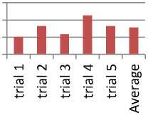
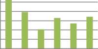
Time taken by individual K-mean algorithm, fuzzy similarity algorithm, and SOM algorithm is presented below in Fig.2, 3 and 4. Average values have been generated by each algorithm. The individual CPU time taken, for clustering, by three of the algorithms is different, as presented in Fig.5.

The comparison of time consumed shows that SOM took maximum time in clustering. Graphical representation of results in Fig.5 shows that comparatively k-mean algorithm is best in terms of CPU time, as clustering is done in lesser time. Fuzzy algorithm also performed satisfactory but SOM took the worst time. And hence it is not suitable for computing missing values (Lu, Ma et al. 2013).

The comparison of time consumed shows that SOM took maximum time in clustering. Graphical representation of results in Fig.5 shows that comparatively k-mean algorithm is best in terms of CPU time, as clustering is done in lesser time. Fuzzy algorithm also performed satisfactory but SOM took the worst time. And hence it is not suitable for computing missing values (Lu, Ma et al. 2013).

Three algorithms for computing mean value were specified previously, now they are combined with k-mean, fuzzy matrix and SOM to get clusters, and performance is analyzed when missing values are substituted in it i.e. constant substitution, mean value substitution, and random value substitution. Following Table.2 and Fig.6 present their combined results .

SOM

■ SOM Trails

i-i  гч  со  ^  ш   си

_ _ _ _ _ ею

ГО    ГО    ГО    ГО    ГО    ГО

Ь Ь Ь Ь Ь  си

• Fig.4.    Average generated by SOM Algorithm

Comparison of Average Time of Algorithms

k- Fuzzy SOM means

□ Average

• Fig.5.    Comparison of Average Time of Algorithms

  K-means

  
  
  
  
  

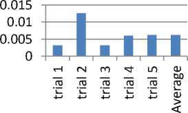
  Fig.2. Average generated by K-mean algorithm

  
  

  Table 2. Clustering Accuracy for Comparison of Average Performance

  	% Missing Value Attributes	K-means	Fuzzy	SOM
  Method 1 Constant Substitution	10	0.842912	.842323	.780717
  	20	.770207	.778559	.722800
  	30	.650338	.813381	.726439
  	Average	.779385	.813381	.726439
  Method 2 Mean Value Substitution	10	.851714	.860034	.795121
  	20	.837110	.833634	.780700
  	30	.838256	.839414	.797277
  	Average	.84529	.846791	.79165
  Method 3 Random Value Substitution	10	.851123	.851123	.790297
  	20	.804928	.808238	.736625
  	30	.789178	.794562	.714089
  	Average	.824828	.827001	.758378

  
  

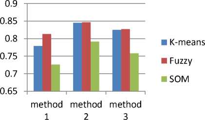
Fig.6. Average Performance Evaluation with Clustering

Comparison of accuracy of clustering techniques, used with proposed algorithms, to compute missing values in dataset concludes that missing values were derived in random fashion. And these missing values were then put together in WDBC dataset. The generated results presented in Fig. 6 were compared with original dataset, hence concluded that evaluated methods for computation of missing values showed that attribute mean produced better results, even the randomized value generation also produced acceptable results. But constant substitution of numeric value produced poor insignificant results. On the other hand, k-mean and fuzzy algorithm performed equally well with regards to CPU time, but SOM based clustering was time consuming as it takes time to train dataset. Hence, data warehouse performance must be improved by data cleaning and pre-processing.

Query optimization is another useful factor to increase data warehouse efficiency. Creation of Materialized Views is one way of query optimization which has been discussed below.

• V. Materlized Views (MVs) for Query Optimization

Knowledge-based systems are used for data analysis, and they are considered essence of data warehouse. The foremost aim of building a data warehouse is to perform an efficient analysis of data in order to strengthen strategic decision making. Online Analytical Processing (OLAP) applications are used to determine patterns in data, trend analysis of particular category data, error detection, as well as they point out dependencies and relationships among data. Therefore, huge amount of heterogeneous data increases the complexity of data, resulting in overhead of processing. To minimize query timing, need of an optimized structure aroused.

Typical queries of data warehouse access massive amounts of data to produce the desired results, but their complexity of nature increases response time (Calvanese, De Giacomo et al. 2012). Materialized views (MVs) proved to be very helpful in increasing the query and processing speed, and are being compatible with tools of database systems. Their query intensive nature makes them suitable for data warehousing environment. When the queries are executed, many join and aggregation functions are performed to complete the transaction, but creation and usage of materialized views eliminates joins and aggregation overhead. The results of transactions are analyzed to understand the problem and to make fast decisions. Materialized views decrease the query processing time when data is accessed from large tables (Mitschke, Erdweg et al. 2014). Materialized views make possible to store results of queries in cache in the form of tables that are constantly updated from time to time, resulting in quicker access. And frequent queries are performed with in no time because of cached table. In addition table can be altered anytime by building indexes against columns, thus increasing the query speed. Materialized Views are implemented in Oracle databases. Three important stages of MVs include: View Design, View Maintenance, and View Exploitation. Following Fig.7 shows the life cycle of materialized views and levels of abstractions, shows how they provide details at certain level. Creation and maintenance of materialized views and their child views are discussed below.

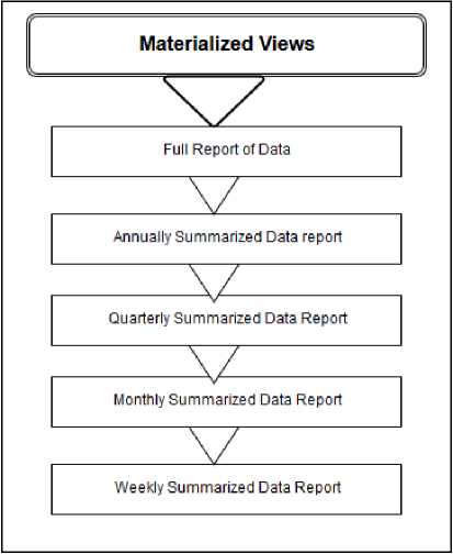
Fig.7. Life Cycle of Materialized Views

• A.    Creation and Maintenance of Materialized Views

Creation of MVs aroused questions that how many materialized views shall be created and what data to be portrayed in MVs. Database administrators define MVs at certain time period and are influenced by access of data. This process continues throughout the whole life cycle of data warehouse activities. If some MVs are not in use, they are dropped from base table and release the space occupied, thus making the data warehouse more efficient and responsive (Folkert, Gupta et al. 2011).

New MVs will be created if there will be more extraction queries. “MiniCon Algorithm” is much suitable in answering queries by utilizing views. Following types of materialized views are used:

• •    Materialized views with aggregates: MVs contain only aggregates performing summarization functions. It includes Sum function, Count Function, Min, Max etc.

• •    Materialized views with Joins: These MVs contain joins which are pre-calculated in advance and then utilized and refreshed on committing the transactions.

• •    Nested Materialized views: One materialized view is based on other materialized views; they are dependent on each other. They complete their working by referencing each other.

• B.    Creation and Maintenance of Child Views

  Once materialized views are created and data is portrayed in it, then child MVs are created (Mitschke, Erdweg et al. 2014). To create child views, all the data types and columns are determined and data dictionaries are retrieved, and aggregation operations are determined. Type of values that are present in columns are scanned, if they are numeric values then they are easily aggregated. Some text values that are referenced, cannot be aggregated e.g. images, audio, videos etc. so textual data is summarized in the form of hierarchies. But to create child views automatically is a very difficult task, due to anomalies in massive data. Once the data is in improved form then it will be an easier task.

Proper and balanced materialized views and child views creation plan is required with higher access frequency rate. And useless MVs shall be removed for optimization purpose, and maximum queries will be satisfied with the help of MVs (Koch, Ahmad et al. 2014).

After the completion of data cleaning and preprocessing, it is important to determine the efficiency of data warehouse, using certain evaluation parameters. Primary Evaluation Attributes have been discussed below.

• VI. Evaluation Attributes and Framewoks

  Evaluation attributes play a significant role in defining the performance of data warehouse after completion of data cleaning process (Philip Chen and Zhang 2014). There are six primary attributes presented below to

analyze the performance of data warehouse:

• A.    Evaluation Attributes

• •    Completeness:  Completeness refers to the

  available data in data warehouse, as data is updated periodically so it may be incomplete, but should be able to satisfy user queries (Rajaraman, Ullman et al. 2012). E.g. names of customers are compulsory but their blood group information is optional so names should be available and optional information could be discarded or updated on later date.

• •    Consistency:  Data  consistency refers to the

synchronized  data  in data warehouse.  The integrated data should not be controversial; it should be consistent across all the departments of an organization (Majchrzak, Jansen et al. 2011). E.g. If a customer has submitted his outstanding bill in one branch of bank, then system should not show the bill status payable in some other branch of bank.

• •    Validity: Validity of data means it is correct in all aspects e.g. Bank account number of a customer is invalid, incorrect numeric values, wrong spellings etc.

• •    Integrity: Integrity means data is free of redundancy, it does not contain any duplicate values, and data is unaltered.

• •    Conformity: The integrated data shall conform to the rules and standards of data warehouse, it should correspond to the proper format, language etc.

• •    Accuracy: Accuracy means that data should correspond to the real world values e.g. Bank balance of customer should be accurate; it should not contain any ambiguous values.

After the completion of all data warehouse processes, some frameworks can be used for the maintenance of Data Warehouse and its efficient working. Four most commonly used frameworks have been discussed below.

• B.    Frameworks

  The task of collecting data from heterogeneous source systems, cleaning, and transforming the data into single depiction and loading the associated data into a target system can be prepared by using single or combination of products (Prerna S. Kulkarni & Dr. J.W. Bakal) (Satterthwaite, Elliott et al. 2013). Some frame works have been presented previously; four efficient ones have been presented below in Table.3. Following frameworks, not only include steps for data cleaning, but also have been compared with each other.

Table 3. Comparison between Frame works

Frame works	Explanation	Cycle	Advantages	Disadvantages
1st: TDQM Frame work	Continuous data quality improvement	•     Define •    Measure •     Analyze •     improve	•     easy to implement •     easy to manage •     data cleaning from user perspective	•     only focused on characterizing data quality research and method instead of data cleansing
2nd Frame-work	•     Rule based •     Rule scheduling •    Log management	•     Data access interface •     Data quality analysis •     Data transformation •     Result assessment	•     Unified design (all data cleaning process performs in single place) •     Unified data extraction interface for single source and multisource data •     To maintain complete information of process Log management is done	•     Data quality process should not be repeatedly done •    Process must be sequential •    Process should perform in single go, not in iterative steps
3rd Frame-work	•     Reduce time •    Reduce complexity of mining process •     Increase data quality	•     Attribute selection •     Formation of tokens •     Clustering algorithm selection •     Computation of similarity among various attributes •     Elimination function selection •    Merge	•     Data cleansing rules can be modified easily	•     Limited to duplicate records elimination •     Less interactive
4th Frame-work	User model- abstraction from real model	•     Access to database objects for user model •     Definition of user model •     Definition of quality model based on user model	•     Simple •     Interactive •     Less steps	•    Requires user model to cleansing work •     Lengthy process •     Does not allow selection of attributes •    Wastage of time •    Wastage of resources

Framework can be selected on the basis of the requirements and benefits (Mohamed, Kheng et al. 2011). These frameworks ensure following data quality measures.

• •   Completeness (of values)

• •   Accuracy (to the Source)

• •    Validity (Business rule conformance)

• •    Precision

• •    Non-duplication (of occurrences)

• •    Derivation Integrity:

• •    Accessibility

• •    Timeliness

Comparison of the tools, used for data warehouse processes, is also an important factor, so that most efficient tool can be used to improve the data warehouse performance. Following section discusses the various data warehouse tools in detail.

• VII.    Tool Support

Various tools are accessible with in the market that are used to accomplish acute tasks involved in process of data cleaning. Transformation tools are also available in wide range for data mapping and field mapping. There may be open-source or commercial (proprietary) tools available requiring specific API’s (Application Program Interface). Some tools deal with specific phases such as cleaning names or address fields, some tools eliminate redundancy, some tools work for particular domains only, some tools may be customized according to user requirements. ETL tools also exist, mainly performing pre-processing activities separately or in collaboration with additional jobs. But, contrary to this, ETL tools provide limited performance due to their need of proprietary API’s and also they are not compatible with other tools due to lack of Meta data (Majchrzak, Jansen et al. 2011). These tools are mainly categorized in following sub-sections:

• A.    Analysis Tools

  Data Analysis tools are further categorized in two types based on their characteristics (Rahm and Do 2000):

Data profiling tools: These tools provide an overview of the wholesome attributes of the data, either revealing critical parts of accumulated data. They analyze numeric attributes and their values within specified range and determine dependencies and duplication.

In addition, they perform summarizations and aggregations processes to get related information. Gathered information is then all set for decision making.

For example, “MIGRATION ARCHITECT” identifies the real meta-data properties. Additionally it helps in schema development. “ALTERYX” provides a platform for strategic decision making and also high lights the inconsistencies among the data.

Data mining tools: These tools are complied with business intelligence techniques and deliver effective and reliable answers to business queries that were previously very difficult to obtain by even experts (Rahman 2016).

They make available such hidden patterns from massive data that increase information reliability (Cios, Pedrycz et al. 2012). For Example, “YALE” (open source) is predictive analytic tool offering statistical comparison facilities with template based approach. “WEKA”(open source) is non Java- based tool that can be integrated into other applications and thus providing predictive modeling on meta data components (Singhal and Jena 2013).

• B.    Specialized Data Cleaning Tools

These tools are designed according to customer requirements and accommodate the cleaning tasks accordingly. These tools are designed in such a way that they clean data of a particular domain, thus they are domain specific.

For Example, “PURE INTEGRATE” and “TRILLIUM” are domain specific, work on pre-defined rules. Once data is cleaned it will be easier task to perform transformations. “DATA CLEANER” provides various fascinating features i.e. detects duplications, provides standardization with constant data health monitoring and thus providing a quality eco system for cleaning, that is comprised with ability of plug and can be integrated into other programs due to its ease of use.

• C.    ETL Tools

Open source and commercial tools for ETL processes are available in market in wide range. For example, “EXTRACT”, “DATA TRANSFORMATION SERVICE” provided     by     Microsoft,     “WAREHOUSE

ADMINISTRATOR”. They contain a built-in DBMS that manages internal as well as external sources, source mappings to components, source codes, schemas etc. in a constant way. Firstly, data is extracted from OLTP (Online Transaction Processing) system, it is then cleansed with various tools and transformations are performed on clean data with the help of mapping rules that are already specified in its schema(Rahm and Do 2000). They provide simple and straight-forward Graphical User Interfaces so that users may be able to correspond easily. ETL tools deal with whole ETL process, they does not perform cleaning as a separate process but can integrate API’s of cleaning tools in it, thus providing better results. They deal with instance related and schema related problems of data cleaning as well.

• VIII.    Conclusion and Future Work

Data Cleaning is most significant process in Data Warehousing, as whole performance rely on it. A survey of Cleaning Process and problems that are involved in ETL stage of Data Warehouse has been presented. Data Pre-processing is one of the main stage of Data Cleaning. Classical and Advanced Pre-processing types have been discussed in the paper. Classical Pre-processing has data fusion, cleaning and structuration phases. Data Cleaning Problems have been discussed in the paper, which lead to disastrous dilapidation in performance of data warehouse. Data Cleaning types and sources have been studied thoroughly. These sources include single source and multi-source problems. Each source has schema and instance level. Then approaches Record Matching and Data repairing (Fan, Ma et al. 2014) have been presented, that are used to eliminate data de-duplication and enhance the quality of data. With the help of these two approaches designers are able to “clean” the data, which is further utilized for strategic decision making, thus enhancing the quality of data warehouse as well.

Missing value problem is toughest to handle. Reasons and types of missing data have been studied and mostly used techniques to handle them have been discussed, like ignoring of missing data tuple, using global constant, using attribute mean and data mining algorithms. Three major techniques used for pre-processing of missing values are Constant Substitution, Mean Attribute Value Substitution and Random Attribute Substitution. Pseudo codes have been presented for these three techniques in the paper. Not only many data mining algorithms have been presented for its solution but also they have been evaluated on the basis of certain evaluation attributes, to determine the most efficient technique. Dataset of WDBC has been utilized for the evaluation of algorithms. Accuracy results for algorithms (k-means, Fuzzy and SOM) have been compared and presented in tabular and graphical form for easy visualization. K-means algorithm comparatively is best in CPU time as clustering is done in least time. Fuzzy Algorithm also performed satisfactory results but SOM algorithm takes worst CPU time. K-means, fuzzy and SOM algorithms have been combined with above mentioned three substitution methods for missing values handling to improve the performance and applied on same dataset of WDBC. New results showed that attribute mean substitution method produced best results, randomized value method produced acceptable results and constant substitution method produced poor results in all.

Materialized Views (MVs) approach is another way to increase performance of data warehouse, by optimizing the queries. Creation and maintenance of materialized views have been discussed in paper, with thorough explanation of its life cycle. Three types of MVs also have been presented: MVs with aggregates, MVs with Joins and nested MVs. Advantages of using MVs for time saving have been mentioned along with the complexities and difficulties in its creation.

Parameters required to analyze the efficiency of warehouse, have been presented, including six primary attributes like completeness, consistency, validity, integrity, conformity and accuracy.

Evaluation Parameters further act as the base for developing frameworks for the maintenance of warehouse. Four most important frameworks have been explained and each framework’s cycle, advantages and disadvantages have been provided to compare with other frameworks.

At the end, analysis tools, specialized data cleaning tools and ETL tools have been discussed, to improve the implementation process. Data Analysis tools types: data profiling tools and data mining tools also have been discussed. These tools have been compared with each other on the basis of their functionalities. Each tool’s most commonly used examples have also been mentioned.

All these approaches lead to the performance improvement of warehouse. However, data profiling techniques still need to be addressed as they are a necessary part in cleaning process. On the other hand, cleaning of corrupted data requires some iterative and probabilistic models as they can efficiently clean the data (Fan, Ma et al. 2014). There are certain limitations to the present work, cleaning of multiple relations that involve dependencies is much needed to be explored in future. More optimizations techniques still need to be discovered to enhance the efficiency of algorithms.