Data-driven Approximation of Cumulative Distribution Function Using Particle Swarm Optimization based Finite Mixtures of Logistic Distribution

Author: Rajasekharreddy Poreddy, Gopi E.S.
Journal: International Journal of Intelligent Systems and Applications @ijisa
Article in issue: 5 vol.16, 2024.
Free access
This paper proposes a data-driven approximation of the Cumulative Distribution Function using the Finite Mixtures of the Cumulative Distribution Function of Logistic distribution. Since it is not possible to solve the logistic mixture model using the Maximum likelihood method, the mixture model is modeled to approximate the empirical cumulative distribution function using the computational intelligence algorithms. The Probability Density Function is obtained by differentiating the estimate of the Cumulative Distribution Function. The proposed technique estimates the Cumulative Distribution Function of different benchmark distributions. Also, the performance of the proposed technique is compared with the state-of-the-art kernel density estimator and the Gaussian Mixture Model. Experimental results on κ−μ distribution show that the proposed technique performs equally well in estimating the probability density function. In contrast, the proposed technique outperforms in estimating the cumulative distribution function. Also, it is evident from the experimental results that the proposed technique outperforms the state-of-the-art Gaussian Mixture model and kernel density estimation techniques with less training data.
Cumulative Distribution Function (CDF), Probability Density Function (PDF), Logistic Mixture Model (LMM), Particle Swarm Optimization (PSO), Extreme Learning Machine (ELM), Interior-point Method
Short address: https://sciup.org/15019515
IDR: 15019515 | DOI: 10.5815/ijisa.2024.05.02
Text of the scientific article Data-driven Approximation of Cumulative Distribution Function Using Particle Swarm Optimization based Finite Mixtures of Logistic Distribution
Published Online on October 8, 2024 by MECS Press
Density estimation plays a crucial role in understanding and characterizing the behavior of signals in fading wireless channels. By accurately estimating the density of signal strength variations, we gain valuable insights into the statistical properties of the channel. This knowledge is instrumental in designing robust communication systems that can adapt to changing channel conditions. Density estimation enables us to model the fading phenomena, predict signal behavior, and optimize system parameters to ensure reliable and efficient wireless communication. It also aids in the development of advanced modulation, coding, and equalization techniques that mitigate the effects of fading, ultimately enhancing the quality and performance of wireless networks.
Most density estimation techniques attempt to approximate the Probability Density Function (PDF), which is then summed or integrated to yield the Cumulative Distribution Function (CDF). As a result, in most cases, a closed-form expression for the CDF cannot be obtained. The closed form expression of the CDF is critical in calculating performance metrics such as outage probability [1, 2], detection probability, False Alarm Probability, and Bit Error Probability in wireless fading environments [3]. As a result, studies have been carried out to obtain the closed-form expressions for the
PDF and CDF of fading distributions [3–6]. In [3], authors have expressed the CDF of "quadratic-form" receivers over generalized fading channels with tone interference in the form of a single integral with finite limits and integrand composed of elementary functions. The authors of [4] derived the exact closed-form expressions for the bivariate Nakagami-m cumulative distribution function (CDF) with positive integer fading severity index m in terms of a class of hypergeometric functions. Obtaining the closed form expression of CDF of Bivariate Gamma Distribution with arbitrary parameters is studied in [5]. Authors of [6] used Berry-Esseen theorem and the method of tilted distributions to derive a simple tight closed-form approximation for the tail probabilities of a sum of independent but not necessarily identically distributed random variables. Also, CDF can be used to generate the samples of the distribution of the data which can be used for data augmentation. Authors of [7] and [8] have proposed nonparametric and bivariate nonparametric random variate generation and using a piecewise-linear CDF to generate the data. The closed-form expressions of the PDF and CDF of the many fading distributions are proposed as a function of complex functions (such as hypergeometric functions, q-functions, error functions, etc.,). For example, the PDF of the κ - μ distribution is expressed in terms of a modified Bessel function, and the CDF is expressed in terms of a generalized Marcum-Q function in [9]. Hence, we considered a novel technique of obtaining the closed form approximate of CDF using the finite mixtures of Logistic Distribution. The finite mixtures of Logistic distribution are referred to as Logistic Mixture Model (LMM) in the rest of the paper. Since the LMM cannot be modeled using the Maximum likelihood estimator, we proposed two computational intelligence techniques.
The main contributions of this paper are
• To estimate the CDF using finite mixtures of the logistic distribution. This results in a closed-form expression for the estimated CDF, which is expressed in terms of simple exponential functions.
• To use computational intelligence techniques such as particle swarm optimization or extreme learning machine to determine the parameters of the mixtures of the logistic distribution.
2. Related Works
3. LMM Using Multivariate Logistic Distribution
The rest of the paper is organized as follows. Section 2 introduces the LMM using the Multivariate Logistic distribution. Section 3 describes the proposed algorithms to approximate the CDF. Section 4 presents the experimental results on the effectiveness of the Mixtures of the Logistic distribution using the proposed algorithms. Section 5 provides the conclusion on the observations.
Researchers have been continuously developing methods for data-driven probability distribution estimation. Addressing the computational challenges of large, multidimensional datasets, one approach focuses on efficient calculation of the empirical cumulative distribution function (Empirical CDF) [10]. This technique, employing lexicographical summation and divide-and-conquer methods, paves the way for faster kernel density estimation for complex data.
Beyond efficiency improvements, alternative estimation techniques are being explored. Moving Extreme Ranked Set Sampling is a method used to estimate both the CDF and a reliability parameter, offering advantages over traditional approaches like simple random sampling [11]. Extreme Learning Machines present a competitive alternative for PDF and CDF estimation. Leveraging their low computational cost and random hidden layer assignment, ELMs are particularly attractive for large datasets [12]. A fast kernel density estimator based local linear estimate have shown their efficiency in estimating the conditional CDF in dependent functional data case [13].
Looking at more recent advancements, data-driven deep density estimation emerges as a powerful tool. Promising accurate and efficient PDF estimation regardless of data dimensionality or size, DDE offers advantages but may require access to the original PDF in some form during the estimation process [14]. Another approach tackles classification problems in a unique way. Instead of directly analyzing empirical data, this method estimates the underlying probability distribution through the Fredholm equation [15]. This approach offers a distinct perspective on data-driven probability estimation.
Different variants of the multivariate logistic distribution were proposed in many research papers. In this paper, the multivariate logistic distribution of the type I proposed by Malik et. al. [16], with some arbitrary center μ and scale parameters S is considered to build the mixture model. The joint cumulative distribution function of x 1 , x2,...,xn which follow logistic distribution is defined as
L(x1,X 2 ,...,xn|p,S) =
1 ^-P (- (jj
The corresponding joint probability density function is
1(Х 1 ,Х 2 ,...,Хп11Л,1) =
n!exp ( - Z jUg^ n " = i^ [1 +S " = i ex P (-^)]
where /л = (/ 1 ,/ 2 ,...,/п) and S = (o 1 , o' 2 ,...,o'n). Let x = [x1,x2,...,xn]rbe the random vector with the CDF Fx(x; 0), then Fx(x; 0) can be written as linear superposition of the multivariate logistic distributions in the following form
F x (x|0) = SL 1 ^ k L(x;/k, S k )
where K is the number of mixture components, 0 = [п, ц,2], п = [я 1 , n2, ..., я „ ], 0 < ?rk< 1 and £ £=1 nk = 1.
For k = 1,2,...,K,/i = [/ 1 ,/ 2 ,...,/iK ] , S = [^ 1 ,^ 2 ,...,^ ^ ] and /k = (/k ,/ 2 ,...,/ ” ) e ^ ” , Ek =
(o^ ,o k ,..., o’2 ) e (0, от) ” . The corresponding PDF of X, which can be obtained by differentiating Fx(x; 0), is
fx(x|0) = ZL 1 ^ kK x;/ k ,S k )
Z.Q. Shi et al. [17] showed that the LMM mentioned in equation (3) is shown to be identifiable. But the maximum likelihood estimator cannot be used to model the parameters of the (3), since the closed-form expressions cannot be obtained for μ and Σ . Hence, (3) is solved in a semi-supervised manner. The proposed algorithms to model the parameters of LMM are explained in section 3. The modeled parameters can be used to estimate the cumulative distribution function of x.
4 . Proposed Algorithms to Model the Lmm
In this section, we present two algorithms to model the parameters of the LMM. They are
-
• Extreme Learning Machine (ELM) framework using the interior method.
-
• Multilevel Particle Swarm Optimization (Mu-PSO).
The parameters of the LMM are computed by the two algorithms in a semi-supervised fashion. The basic idea of the proposed algorithms is to use the empirical approximation of the CDF (also known as empirical CDF) as the target value and consider the Mean Square Error (MSE) as the objective function which must be minimized. The empirical CDF of some arbitrarily uniformly distributed points is computed based on the available data. These arbitrary points
Мх0
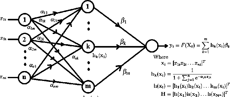
Fig.1. Single hidden layer feed-forward network (SLFN)
and the obtained Empirical CDF values are considered input-target pairs to compute the parameters (output weights) of the ELM and the optimum particle in the swarm of the Mu-PSO.
The Empirical CDF of an arbitrary data point x is obtained by
/(x) =
Number of available data samples < % Total number of available data samples
The x and I(x) pair are assumed as the input and target values of the proposed algorithms.
-
4.1. Modeling LMM Using Interior Point Method in ELM Framework
In this section, (3) is modeled using the interior point method in the ELM framework. The individual mixtures L(x; yk, Sk) in (3) are considered as the hidden layer activations and the mixing probabilities ik as the output layer weights of a Single hidden Layer Feed-forward Network. The Empirical CDF values I(x) of the corresponding input data points x are considered as the target of the SLFN. The details of the ELM algorithm are presented in section 4.1.1.
-
A. Extreme Learning Machine (ELM)
An Extreme Learning Machine (ELM) is a Single hidden Layer Feed-forward Network that randomly chooses hidden node weights and analytically determines the output weights [18]. Fig. 1 shows the network structure of SLFN where a j k,j = 1,...,n, k = 1,...,K are hidden layer weights, pk,k = 1,2,...,K are output layer weights. The output y , ,i = 1,...,N corresponding to the input x , = [х 1, ,...,xn , ], for i = 1,...,N is obtained by y , = £k =1 hk(x , )pk. The output can be represented in matrix form for all inputs x , ,i = 1,...,W as,
У = HP (6)
Algorithm 1 : Extreme Learning Machine (ELM)
Given a training set X = {(x , ; t , )|x , £ ^n; t , £ ^; i = 1,...,Wn}, activation function hk ( xi ) , number of hidden nodes K and a target T = [t 1 ,..., tN ]T .
Step 1: Randomly assign input weights a j k,j = 1,...,n,k = 1,...,K.
Step 2: Compute the hidden layer output matrix, H.
Step 3: Find the output weight vector, β as
p = h+t
Step 4: Compute the output of SLFN for a test data, xtest can be found by
y(xtest) = h(xtest)H+T = h(xtest)(HrH) - Hr T where H = [h(x1)h(x2) ...h(xN )]T is the hidden layer activation matrix of all the input samples, h(x,) = [h1(x,), ...,hK (x,)]r is the hidden layer activation vector of the input sample xi, hk (xi) is the activation of the kth hidden node, p = [P1,...,PK ]T , and T = [t1,...,tN ]T. The values of ajk are randomly assigned and the values of вк are computed by minimizing the MSE,
MSE = ||HP - T||2 (7)
The values of β can be computed by solving (7) using the Least Square method as
P = HfT (8)
where H = (HTH)-1 HT is the pseudo-inverse of the matrix H.
-
B. Interior Point Method
The ELM solves its objective function using the Least Squares (LS) method, but the proposed algorithm uses the interior point method to solve the least squares problem, to satisfy the constraints of the probability. The objective function of the ELM algorithm in equation (7) does not impose constraints on the mixing probabilities ik of (3). Hence the ik obtained in the section 4.1.1 may be negative or greater than one [19], which violates the axioms of the probability. To avoid this, equation 7 is solved using the interior point method by imposing the axioms of the probability as constraints. Hence the objective of the ELM approach can be modified by imposing the constraints as follows
/ = min^ MSE = min^ ||L(X; ц,Х)п - T||2 (9)
subject to the constraints, 0 < nk < 1,k = 1, 2,..., K and 2k=i ik = 1. Where X = [x1,x2, . ,xN], /л = (л1,Л2,.. ., л^), S = (S1,...,SN) and i = [11,12, ...^Г.
The objective function in (9) is a linear programming problem with inequality constraints. This problem can be solved using the interior-point methods [20]. Once the parameters л, S, and n are computed using the interior-point method, the CDF of a data point x can be computed using (3). The algorithmic framework of the interior-point method in ELM fashion to model the parameters of (3) is presented in Algorithm 2.
Algorithm 2: Modeling LMM using Interior Point method in ELM framework
Given a training set X = {(x^ t i )|x; £ ^n; t; £ Я; i = 1,...,Nn], activation function
L(x i l^ k ,S k ) =
1 jW)
, number of hidden nodes K and a target T
[t1,..., tv ] .
Step 1: Randomly assign //
k
and
Step 3: Formulate the Optimization Problem as
min^ ||L(X; ц,Е)п - T||2 such that 0 Step 4: Solve for n by minimizing the MSE using Interior Point Method. Step 5: CDF of a test data, xtest can be found by Fx(xtest) = L(xtest; ц, E)n. 4.2. Modeling LMM using Mu-PSO The Mu-PSO proposed in this section is inspired by the Expectation-Maximization technique [21] where the maximum likelihood of a model is obtained by first finding the expectation and then maximizing the model. The objective function mentioned in (9) is solved using the Mu-PSO algorithm in Expectation-Maximization fashion. The detailed algorithm of the Mu-PSO is presented in Algorithm 3. As in the Expectation-Maximization technique, Algorithm 3: Mu-PSO to model LMM Initialize the parameters / and 2 randomly in (-от, от) and (0, ot>) respectively. num_iter - The number of iterations. for l = 1 to num_iter Step 1 - Expectation stage: Compute n; as described in Algorithm 4. The obtained n; will be used as one of the particles of Algorithm 4 in the next iteration. Step 2 - Maximization stage: Compute /; and 2; as described in Algorithm 5. This /; and 2; will be included as one of the particles of the respective swarms in the next iteration. Step 3: Compute the objective function in, /; = / (/;, 2;, n;) Step 4: if (J— - Л) < 10-6 / = /h 2 = 2(,л = n; and break the loop and go to Step 5. end if end for Step 5: Use the values of /, 2 and n to compute the CDF of a test sample x. • Expectation: The values of π are computed using PSO [22-24] algorithm by randomly initializing the μ and Σ. • Maximization: Once π are computed, then the values of μ and Σ can be obtained using PSO. • This process is repeated until convergence of either the parameters or the objective function in (9). The values of π, μ and Σ obtained in the previous iteration are used as one of the particles in the corresponding PSO algorithms. To make sure that π follow the axioms of probability, the absolute value of the next movement of the particles of the PSO used to compute the π are taken, and then normalized so that the sum of each particle equals to one in Algorithm 4. The values of S must range in (0, от), hence the values of E are made positive by taking the absolute values while updating the next position of the population in Algorithm 5. Algorithm 4: Expectation stage Initialization: • Assume the number of particles in the swarm is M, the dimension of each particle is n, c1, c2 are the individual and group learning rates, r1 and r2 are uniformly distributed random numbers between 0 and 1, |.| denotes the modulus and the minimum value of the objective function / is saved in variable min_/ to track the convergence of the algorithm. • Initialize the Mparticle positions of the mixing probabilities, n randomly as nPi, np2,..., пРм and the tentative local decisions taken by the particles randomly as n;dl, n;d2,..., n;dM . The parameters ц and E are fixed with the values obtained in maximization stage. for iteration = 1 to 25 Step 1: Compute the functional values of/(nMm), Vm. Step 2: Find the minimum among / (/, 2, пИт), Vm and declare the particle position as global best, пМд . i.e., nldg = arg minl=i l J^Z^idJ andJ(^,£,nldg) = arg minimi LJ(n,£,nldm). Step 3: Identify the moved next position of the particles. for m = 1 to M nPm_next = |^Pm + cl r1(nldm - nPm) + c2 r2(nldg - npm)| npm_next = npm_next/sum(npm_next) end for Step 4: Assign the current positions of the M particles as np = np _next,Vm and obtain the tentative decision taken by each particle for further movement is obtained as for m = 1 to M ifJ(^,E,nPm_next) ПМт = nPm_next end if end for end for Step 5: Compute the functional values J(^,£,npm), Vm and find the n = arg minm=1 M J(npm ) Algorithm 5: Maximization stage Initialization: • Assume the number of particles in the swarm is L, the dimension of each particle is n, c3, c4 are the individual and group learning rates, r3 and r4 are uniformly distributed random numbers between 0 and 1, |.| denotes the modulus and The minimum value of the objective function J is saved in the variable min_J to track the convergence of the algorithm. • Initialize the L particle positions of the parameters ^ and £ randomly in (-^, <*>) and (0, ^), respectively, as ^ ,^ , — ,ц and £ ,£ ,■,£ , the tentative local decisions taken by the particles randomly as Pl P2 Pl ”1 ^2 ^l ^id^^id^ '",^idL and £ldl,£ld2, — ,£ldL. The mixing probabilities n obtained in the expectation stage are used. for iteration = 1 to 25 Step 1: Compute the functional values of J (^ldl, £ldl, n),Vl. Step 2: Find the minimum among J (^ldl, £ldl, n),Vl and declare the particle position as global best, цы and £ldg. ^ldg,£ldg= argminl=1 L-I(^ldl,£ldl,n) andJ(^ldg,£ldg,n)= minl = 1 L^ld^ld^ Step 3: Identify the moved next position of the particles. for l = 1 to L ^pi_next ^p^ + c3r3(^ldi ^pi) + c4r4(^ldg ^pi) £pl_next = l£pl + c3r3(£ldt - £pj + c4r4(£ldg - £pl)l end for Step 4: Assign the current positions of the L particles as ^pi = ^pi_next and £pi = £pi_next,Vl. Obtain the tentative decision taken by each particle for further movement is obtained as for l = 1 to L if J(^pl_next, £pl_next, n) < J(pldl,£Ш1,л) ^ldi ^pi_next £ldi £pi_next end if end for end for Step5: Compute the functional values J(^pi, £pi, n), Vl and find ^,£ = arg minl=12i^LJ(^pi, £pi, n)
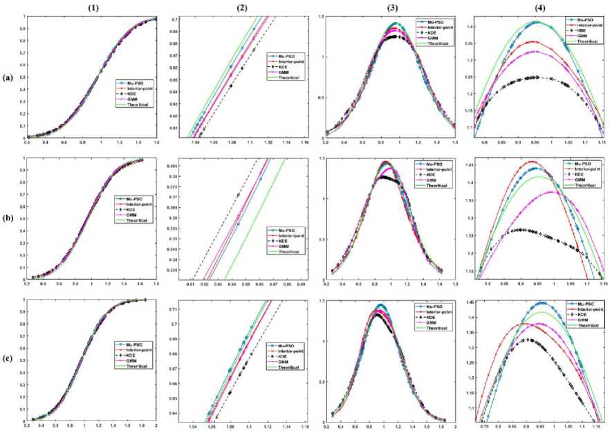
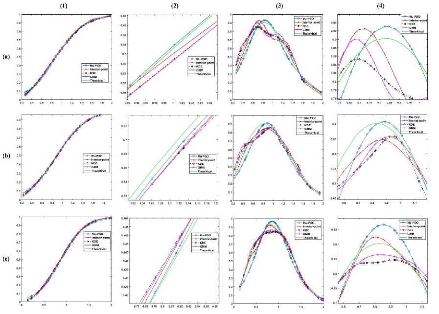
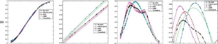
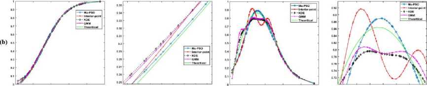
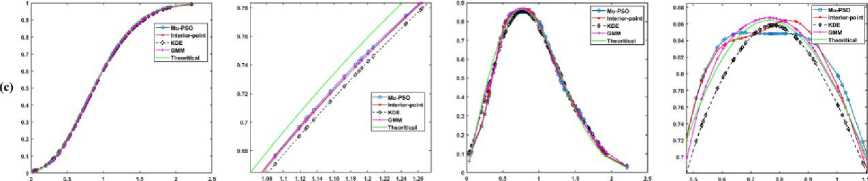
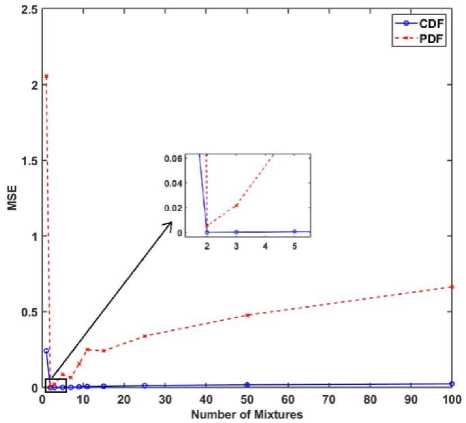
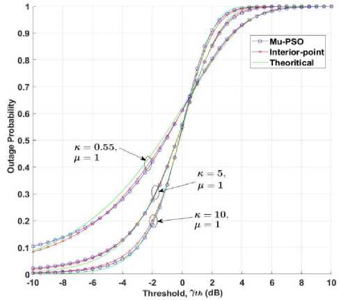
5. Experimental Results In this section, the effectiveness of the proposed algorithms to model the LMM for approximating the CDF is demonstrated using the κ - μ fading wireless environment. The envelope probability density function of the κ - μ distribution is defined using the modified Bessel functions as follows [9], м+1 fR(r) = ——-— rv ехр(-р(1 + к)г2) /м-1 \2м/к(Т+^к)Г\(10) к 2 ехр (рк) where к > 0, м > 0, and Iv[. ] is the modified Bessel function of the first kind and order v. The cumulative distribution function of the κ - μ distribution is defined as FrW = 1-Qv \^2KM,/2(1 + к)рг\(11) where Qv(a,b') =-^~1^^xv ехр(-^-^1г-1[ах] dx(12) is the generalized Marcum Q function [9]. The outcomes of the envelope of the kappa-mu distribution are generated using the in-phase and quadrature-phase components as [9] R = JZM + Pt)2 + Z^ + qd2 (13) where Xi and Yi are mutually independent Gaussian processes with E[Xt] = E[Yt] = 0, E\Xp] = E[Y2] = a2; pi and qi are respectively the mean values of the in-phase and quadrature components of the multipath waves of ith cluster, and n is the number of clusters of multipath. The approximated values of n, pi, qi and σ2 in terms of κ and μ can be written as follows. n = \v] P‘=] к 2п(1+к) qt = Pt 2 1 a2 = ——-2п(1+к) The outcomes of the Gaussian processes Xi and Yi are generated with zero mean and variance σ2. These generated outcomes and the values of n, pi, and qi computed using (14) are used to obtain the envelope R of κ-μ distribution that is defined in (13). For the demonstration purpose of the effectiveness of the proposed techniques, the results are presented for different values of κ and μ. The generated data is divided into train and test data. The train data is used to model the proposed methods to approximate the CDF of the data. The test data is used to check the efficiency of the proposed methods in approximating the CDF of the data and hence the PDF. The performance of the proposed methods is compared with the theoretical values computed using the method proposed by M. D. Yacoub [9], and the estimated values by using the state-of-the-art techniques Kernel Density Estimator (KDE), and Gaussian Mixture Model (GMM). The training of the estimation methods is performed with 500, 100, and2000 numbers of the samples, and the trained algorithms are tested with 100 samples. The number of mixtures used for the proposed interior-point method is 100 since some of the mixing probabilities becomes 0 while solving the equation in (9). The parameters of PSO used in the Algorithm 4 are M = 30, c1 = 0.3, and c2 = 1. The parameters of PSO used in the Algorithm 5 are L = 30, c3 = 0.7, and c4 = 1. We have showcased our results across various combinations of κ and μ values. These different parameter settings yield distinct probability distributions. Specifically, when κ = 1 and μ = 1, it corresponds to the Rician distribution. Conversely, when κ = 0, it transforms into a Nakagami-m distribution with m equal to μ. Fig.2(a), (b), and (c) shows the approximation of the CDF and PDF of the κ-μ distribution for κ = 10 and μ = 1 with the training samples of 500, 1000, and 2000 respectively. Similarly, Fig.3., Fig.4., and Fig.5. demonstrate the approximation of CDF and PDF with different training samples for κ = 5, μ = 1, κ = 1, μ = 1 and κ = 0.55, μ = 1, respectively. It is evident from Fig.2.- 5. (a) that the proposed methods approximate both the CDF and PDF better than compared to the KDE and GMM even when the number of training samples is less. Also, one can see from Fig.2.- 5. (b) and (c), that, as the number of samples increases the performance of the proposed methods is like that of KDE and GMM. However, the proposed method offers a distinct advantage by providing a closed-form expression for the CDF. Fig.2. Comparison of the CDF and PDF estimated using different methods for κ = 10 and μ = 1 with the number of training samples of (a) 500, (b) 1000, and (c) 2000. In each row (1) CDF, (2) CDF zoomed, (3) PDF, and (4) PDF zoomed Fig.3. Comparison of the CDF and PDF estimated using different methods for κ = 5 and μ = 1 with the number of training samples of (a) 500, (b) 1000, and (c) 2000. In each row (1) CDF, (2) CDF zoomed, (3) PDF, and (4) PDF zoomed Fig.4. Comparison of the CDF and PDF estimated using different methods for κ = 1 and μ = 1 with the number of training samples of (a) 500, (b) 1000, and (c) 2000. In each row (1) CDF, (2) CDF zoomed, (3) PDF, and (4) PDF zoomed This closed-form CDF can serve multiple purposes, including calculating outage probabilities and generating data using the inverse of the CDF. The variation in the MSE of the estimated CDF and PDF when compared to the theoretical values with different numbers of mixtures is shown in Fig.6 for κ = 10 and, μ = 1 with 2000 training samples. (1) (2) (3) (4) О 0.5 I 1.5 J 09 0.02 0.04 9 0S 099 9 0 OS I 1.5 2 0.5 0.9 0.T 0.9 0.9 0.5 1 1.5 2 2.8 0.54 0 M 0.53 0.5 042 0Ы 0.96 OSO 9 US I 1.5 2 2 5 0 5 0.5 0.7 0.3 0.9 Fig.5. Comparison of the CDF and PDF estimated using different methods for κ = 0.55 and μ = 1 with the number of training samples of (a) 500, (b) 1000, and (c) 2000. In each row (1) CDF, (2) CDF zoomed, (3) PDF, and (4) PDF zoomed Fig.6. Comparison of the MSE of the estimated CDF and PDF with different numbers of mixtures using Mu-PSO algorithm The optimum number of mixtures that are needed to estimate the CDF of the κ-μ distribution with κ = 10 and, μ = 1 is 2 because the κ-μ distributed data is generated with two independent and identically distributed Gaussian distributions with different variances when μ = 1. Since the closed-form expression of the CDF approximation is a simple exponential function, the outage probability, Pout [1, 2] can be easily computed as Pout = P(x < y^) = ^(yj = £Kk=1TikL(yth-> F^k)(15) The outage probability computed using the proposed methods is compared with the theoretical values proposed in [9]. The outage probability of the κ – μ distribution as a function of the γth (dB) for κ = 0.55 and μ = 1, κ = 5 and μ = 1, κ = 10 and μ = 1 is plotted in Fig.7. 2000 samples of the kappa-mu distribution are used to train the proposed methods in this instance. It can be observed from Fig.7., how close the outage probabilities obtained by the proposed methods are to the theoretical values. Fig.7. Outage Probability at three different combinations of κ and μ
6. Limitations Since the interior-point based ELM method takes the parameters of Logistic distribution randomly, it needs a greater number of mixtures to exactly model the LMM in approximating CDF. The Mu-PSO method needs a smaller number of mixtures when compared to interior point method since it tries to obtain all the parameters of LMM using PSO. However, Mu-PSO method takes more time when compared to interior point-based ELM.
7. Conclusions We have successfully developed closed-form expressions to approximate the CDF and PDF of the κ-μ distribution using LMM. Our comprehensive evaluation reveals that these new approximations outperform current state-of-the-art methods in accurately approximating the CDF and PDF of the κ-μ distribution. Notably, these methods demonstrated impressive accuracy even with a relatively small dataset of just 500 samples. Furthermore, it’s worth highlighting that our presented approaches can be extended beyond univariate data. They can be adapted to estimate the CDF and PDF of multivariate data, offering broader applicability. Additionally, exploring the potential of these techniques to approximate the CDF and PDF of other probability distributions presents an exciting direction for future research.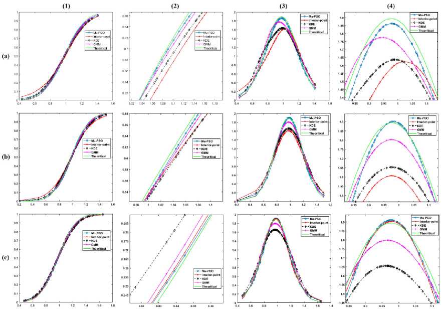
References Data-driven Approximation of Cumulative Distribution Function Using Particle Swarm Optimization based Finite Mixtures of Logistic Distribution
- D. Morales-Jimenez and J.F. Paris, “Outage probability analysis for η − μ fading channels”, IEEE Communications Letters 14 (6) (2010), 521–523.
- M. Milisic, M. Hamza and M. Hadzialic, “Outage Performance of L-Branch Maximal-Ratio Combiner for Generalized κ – μ Fading”, in VTC Spring 2008 - IEEE Vehicular Technology Conference, 2008, pp. 716–731, [10.1109/VETECS.2008.79].
- M.D. Renzo, F. Graziosi and F. Santucci, “On the cumulative distribution function of quadratic-form receivers over generalized fading channels with tone interference”, IEEE Trans. On Communications 57 (7) (2009), 2122–2137.
- F.J. Lopez-Martinez, D. Morales-Jimenez, E. Martos-Naya and J.F. Paris, “On the Bivariate Nakagami-m Cumulative Distribution Function: Closed-Form Expression and Applications”, IEEE Trans. on Communications 61 (4) (2013), 1404–1414.
- N.Y. Ermolova and O. Tirkkonen, “Cumulative Distribution Function of Bivariate Gamma Distribution With Arbitrary Parameters and Applications”, IEEE Communications Letters 19(2) (2015), 167–170.
- J.A. Maya, L.R. Vega and C.G. Galarza, “A Closed-Form Approximation for the CDF of the Sum of Independent Random Variables”, IEEE Signal Processing Letters 24 (1) (2017), 121–125.
- W. Kaczynski, L. Leemis, N. Loehr and J. McQueston, “Nonparametric Random Variate Generation Using a Piecewise Linear Cumulative Distribution Function”, Communications in Statistics - Simulation and Computation 41(4) (2012), 449–468. doi:10.1080/03610918.2011.606947.
- W. Kaczynski, L. Leemis, N. Loehr and J. McQueston, “Bivariate Nonparametric Random Variate Generation Using a Piecewise-Linear Cumulative Distribution Function”, Communications in Statistics - Simulation and Computation 41(4) (2012), 469–496. doi:10.1080/03610918.2011.594532.
- M. D. Yacoub, “The κ−μ distribution and the η−μ distribution”, IEEE Antennas and Propagation Magazine 49 (1) (2007), 68–81.
- L. Nicolas and W. Xavier, “Fast multivariate empirical cumulative distribution function with connection to kernel density estimation”, Computational Statistics and Data Analysis, 162 (2021), 1-16.
- E. Zamanzade, M. Mahdizadeh and H.M. Samawi, “Efficient estimation of cumulative distribution function using moving extreme ranked set sampling with application to reliability”, AStA Advances in Statistical Analysis, 104 (2020), 485-502.
- C. Cristiano and M. Danilo, “An Extreme Learning Machine Approach to Density Estimation Problems”, IEEE Transactions on Cybernetics, 47 (10) (2017), 3254-3265.
- M. A. Ibrahim, C. E. Zouaoui, L. Ali and R. Mustapha, “kNN local linear estimation of the conditional cumulative distribution function: Dependent functional data case”, Comptes Rendus Mathematique, 356 (10) (2018), 1036-1039.
- P. Puchert, P. Hermosilla, T. Ritschel and T. Ropinski, “Data-driven deep density estimation”, Neural Computing and Applications, 33 (2021), 16773-16807.
- M. X. Zhu and Y. H. Shao, “Classification by Estimating the Cumulative Distribution Function for Small Data”, IEEE Access, 11 (2023), 41142-41152.
- H. J. Malik and B. Abraham, “Multivariate Logistic Distributions”, The Annals of Statistics 1 (3) (1973), 588–590.
- Z. Q. Shi, T. R. Zheng and J. Q. Han, “Identifiability of multivariate logistic mixture models”, 2014, Preprint at https://arxiv.org/abs/1208.3546.
- Q.Y.Z. G.B. Huang and C.K. Siew, “Extreme learning machine: Theory and applications”, Neurocomputing 70 (2006), 489–501.
- C. Cervellera and D. Macciò, “An Extreme Learning Machine Approach to Density Estimation Problems”, IEEE Trans. on Cybernetics 47(10) (2017), 3254–3265.
- S.J.W. F.A. Potra, “Interior-point methods”, Journal of Comp. and Appl. Mathematics 124(1) (2000), 281–302.
- C. Bishop, “Mixture models and EM”, in Pattern Recognition and Machine Learning, Springer, New York, 2006, pp. 423–459.
- J. Kennedy and R.C. Eberhart, “Particle swarm optimization”, in IEEE International Conference on Neural Networks, Vol. 4, IEEE Service Center, Piscataway, NJ, 1995, pp. 1942–1948.
- E.S. Gopi, “Artificial Intelligence”, in Algorithm Collections for Digital Signal Processing Applications using Matlab, Springer Dordrecht, Netherlands, 2007, pp. 1–8.
- P. Rajasekharreddy and E.S. Gopi, “Improvement of accuracy of under-performing classifier in decision making using discrete memoryless channel model and Particle Swarm Optimization”, Expert Systems with Applications 213, pp.1-12.
