Data Mining of Students’ Performance: Turkish Students as a Case Study

Published Online August 2015 in MECS

Data mining is a technique that enables the discovery of useful information from data, and it is also sometimes referred to as knowledge discovery. The goal of this process is usually to mine the patterns, associations, changes, anomalies, and statistically significant structures from large amounts of data [1].

More precisely, data mining refers to the process of analysing data in order to determine patterns and their relationships [2]. Different approaches can be applied to the problem of data mining, but the particular aim (e.g. classification, identification, changes etc.) and nature of data are important factors in the decision of the system used to explore data. Data mining techniques model data, such that underlying relationships between attributes can be discovered and applied to new data for some task specific purposes. Several data mining techniques have been successfully applied to different problems ranging from biological data analysis, financial data analysis, transportation, and forecasting.

Some of the common approaches to data mining include decision trees, rule induction, nearest neighbour clustering, artificial neural networks, genetic algorithms etc. [3]

The major motivation behind data mining is that there are often information “hidden” in the data that are not readily evident, which may take enormous human effort, time and therefore cost to extract [4]. Furthermore, with exponential increase in the processing power of workstations (computers) now available today, it is possible for data mining search algorithms to quickly filter data, extracting significant and embedded information as required.

The ability to extract important embedded information in data suffices in many situations, helping organizations, companies, and research analysts make significant progress on different problems and decisions that are based on more information.

The problem of evaluating students’ performance relative to some critical factors that seem to significantly affect the possibility of having to repeat a course has been reviewed in this research. This is generally a complex problem considering the number of such factors that contribute to the success or failure of students in a course. This research explores the ability to mine available data using neural networks, and therefore from the information acquired be able to associate what factors are more important than others in the success of students, predict the number of times a student will have to repeat a course before passing, and how those critical factors can be fine-tuned for effecting better performance of students.

The remaining sections of this research present some brief insight into artificial neural networks, their designs, training and testing to achieve the prediction problem as stated above.

• II.    Related Work

Data mining of students' performance has been considered by many researchers; Baradwaj and Pal [5] applied the ID3 version of the decision tree algorithm to predict End Semester Marks (ESM). They considered as factors that are related to the students end of the semester marks such as the Prevoius Semester Marks (PSM), Class Test Grade (CTG), Seminar Performance (SEP), Assignment (ASS), General Proficiency (GP), Attendance (ATT), and Lab Work (LW). After running the decision tree algorithm, they were able to obtain some set of IF-THEN rules for the prediction of students ESM into first, second, third, and fail.

Dorina Kabakchieva [6], in her work applied various algorithms such decision tree, Bayesian classifiers, K-nearest neighbour, and rule learners to model the students’ performance from collected data. It was reported in the work that while these classifiers suffice for the data mining problem, the best result obtained from any of the classifiers or algorithms was 75% accurate, which is relatively poor considering the importance of the task. .i.e. prediction of students’ performance.

Osofisa et al. [7], also in their work compared the capability of artificial neural networks to decision trees in modelling the performance of enrolled students at their institution, university of Ibadan, Ibadan, Nigeria. It was established that the neural network model outperformed the decision tree model on both the training and test data. The best performance was reported for the multilayer perceptron model with classification accuracies of 98.2639% and 60.1626% for the training and test data respectively.

In this research, we exploited the power of artificial neural network to learn such a complex task of predicting students’ performance from the somewhat fuzzy data obtained from completed questionnaires by 5820 students from Gazi University, Ankara, Turkey; while using the cross-validation technique to guide the trained networks to obtaining far better generalization results on the test data. This work differs from other works in that all the attributes considered to predict the performance of a student are based on the student’s current academic experience at the school; previous experiences and academic excellence are of no effect. This approach creates a fair basis for the assessment of learning structure and academic motivation that an institution offers to students, irrespective of their past educational backgrounds.

• II.    Artificial Neural Network (ANN)

• A.    Preliminaries

An Artificial Neural Network (ANN) is a mathematical model that tries to simulate the structure and functionalities of biological neural networks [8]. These computational units are commonly referred to as artificial neurons and they are the basic building blocks of all neural networks. Graupe, in his book, described artificial neural networks as computational networks, which attempt to simulate, in a gross manner, the network of nerve cells (neurons) of the biological (human or animal) central nervous system [9].

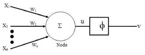
Fig. 1. Artificial neuron

A neural network's ability to perform computations is based on the hope that we can reproduce some of the flexibility and power of the human brain by artificial means [10].

Artificial neural networks simulate the brain in two core areas which are structure and functions; neural networks possess features which are at least roughly equivalent to the ones found in biological neurons. Artificial neural networks are an attempt at modelling the information processing capabilities of nervous systems [11]. The the artificial neuron is shown below, and the equations expressing the relationship between the inputs and the output.

u = E wx                      (1)

v = Ф ( u )                                    (2)

Where, i is the i-th node or neuron, j is the index of the inputs, wij is the weight interconnection from input j to neuron i, x1, x2, ….., xn, are the inputs to the neuron, w1, w2,…., wn, are the corresponding weights to the neurons, u is the total potential, ϕ is the activation which can be used to introduce nonlinearity to the relationship between the inputs and output, and v is the output of the network. Note, that various functions are used as activation functions or transfer functions; common functions in neural networks include log-sigmoid, tan-sigmoid, Signum, linear, Gaussian etc.

• B.    Back Propagation Neural Network (BPNN)

These are multilayer neural networks, which have the ability to learn the relationship between the inputs and outputs by adjusting the memory (weights) of the network each iteration. The back propagation algorithm is a supervised learning algorithm, which means the networks are supplied with the training examples and the corresponding desired or target outputs. The network compares the actual computed output against the desired output and generate an error signal, e, is propagated back into the network for the update of weights, this is process is executed each epoch till the desired error level is reached or maximum number of epochs has been reached.

Generally, multilayer networks have an input layer, output layer and one or more hidden layers; hidden layers are the layers between the input and output layers. It is to be noted that the number of neurons in each layer varies in accordance to the dimension of the input (the number of attributes that make up one training sample), the nature of the problem to be solved (e.g. regression, classification etc.) determines the number of neurons in the output layer, while the suitable number of neurons in the layer is usually obtained heuristically during the training phase of these networks.

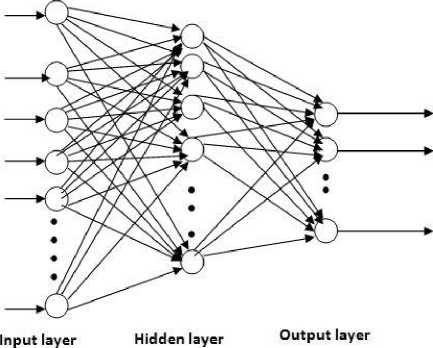
Fig. 2. Back propagation neural network error = actual output - desired output     (3)

actual output = u = ^ w^Xj              (4)

The figure above shows a typical back propagation network with a single hidden layer, the goal of the back propagation algorithm is minimize the error towards the desired set value.

Let the actual output of the network when pattern k is supplied be uk, and the desired output be dj, then the error signal due to pattern k becomes ek = vk - dk

Using the standard gradient descent method to minimize the error, the individual error signals at the output are accumulated over all the training samples using MSE (Mean Square Error) approach, and the error signal is propagated back to update the network weights correspondingly.

kk

MSE = e = £ e , ² = £ ( v , - d , )²          (6)

*       de

Awj = d Wj

The equations that can be used to update the weights of the neurons in a back propagation neural network are given below.

• 1.    Initial weights and thresholds to small random numbers.

• 2.    Randomly choose an input pattern x(u)

• 3.    Propagate the signal forward through the network

• 4.    Compute δ i ^L in the output layer (o i = y i ^L)

  S f = g '( h f )[ d f — y L ]

  
  
  
  

• 5.    Compute the deltas for the preceding layers by propagating the error backwards.

• 6.    Update weights using

• 7.    Go to step 2 and repeat for the next pattern until error in the output layer is below the pre-specified threshold or maximum number of iterations is reached.

Where h i ^L represents the net input to the i-th unit in the l-th layer, and g’ is the derivative of the activation function g.

s i = g '( h i ) ^ W j^Y S ^lj*^Y             (9)

For l = (L-1),…….,1.

A w lj = nS' y r ¹                   (10)

Where w j are weights connected to neuron j, x j are input patterns, d is the desired output, y is the actual output, and η (0.0< η <1.0) is the learning rate or step size [12].

Usually, another term known as momentum, α (0.0< α<1.0), is at times included in equation 1 so that the risk of error gradient minimization getting stuck in a local minimum is significantly reduced [13].

• C.    Radial Basis Function Network (RBFN)

The RBF network is a universal approximator, and it is a popular alternative to the MLP, since it has a simpler structure and a much faster training process [14]. These networks basically are in design much like the back propagation networks, except that they generally have 1 hidden layer. Furthermore, the approach to updating the weights in these networks are quite different from the back propagation networks.

Haykins in his work, noted that these networks can be seen as function approximators when inputs are expanded into a higher dimensional space; while the goal of designed networks will be to find the line of best fit during training for the data set [15]. These networks have as hidden layer activations non-linear activations (called radial basis functions), and the outputs being the linear combination of the radial basis functions.

This approach is so credible when we consider covers' theorem which suggests that when patterns dimensionality are increased, then the probability of achieving linear separation also increases. A brief insight into the theorem is described below.

If we input patterns x1, x2, x3, ….., xm, for which all patterns belong to two classes, say Ca and Cb. Let the function of the patterns be ϕ, then separability is achievable given the conditions below.

• 1.    If W T ф (X ) >  0 ,then x belongs to class Ca

• 2.    If W T ф (X ) <  0 ,then x belongs to class Cb

• 3.    Φ (x) must be a non-linear function

• 4.    The dimension of hidden space must be greater than the dimension of input space

• 5.    W T ф (X ) = 0 defines the equation of the separating hyperplane.

Where w and wT are the weights and weight transpose vectors of neurons, and ϕ is the nonlinear activation function.

If all the above conditions hold, then the probability of achieving separability increases towards 1 significantly. Although there exist variations of the radial basis function networks, owing to considerations such as regularization and optimization; the basic training and update rule remains invariably the same as discussed below.

During training, hidden neurons are centred at some selected points in the training data; approaches involved in achieving this include randomly fixed centre selection, k-means clustering, and orthogonal least squares [16]. The output of each neuron can be seen as the vector distance w and x which is usually obtained using the Euclidean distance approach [17]; the backbone of radial basis function networks being the ability to optimize such distances for neurons such that the distance between w and x for each neuron is minimized. The equations describing the idea which can also be seen as an interpolation problem are given below.

• 1.    Say we have data such that (x^m, o^m) , where x^m and o^m represent input patterns centred on hidden neurons and output targets respectively; for 1 ≤ m ≤ k , where k is the number of hidden neurons.

• 2.    To obtain a function, we use the Euclidean distance parameter below.

• 3.    f ( x ) = ∑ w_m φ ( x - x^m )                  (11)

k

m = 1

It can be seen from equation 11, the nonlinear function, ϕ, applied to the Euclidean distance; there are generally various types of functions used but the most commonly used is the Gaussian function. This is so in view of the way this function responds to the changes in the Euclidean distance between the neuron centres and the input patterns. The equation below describes the Gaussian function [18].

• - r ²

φ ( r ) = e ^{2 σ} ,                                 (12)

Where, r = x - x^m and σ controls the smoothness of the Gaussian curve.

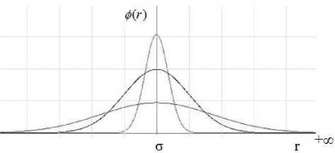
Fig. 3. Gaussian function

From fig.3, the Gaussian suitability can be seen in that as r → ∞ , the value of ϕ(r) decreases and as r → 0 , ϕ(r) approaches it maximum value, 1; hence the Gaussian function is said to be local to the centre vector. The three curves in fig.3 show different Gaussian function curves obtained for different values of the smoothing parameter,

σ, which is also sometimes referred to as the spread constant. Each epoch, the weights of the neurons are updated such that are decreasing.

• II I. Data Analysis and Processing

• A.    Input Data

The data that were used in this work to validate the power of neural networks in data mining and the prediction of how many times a student will repeat a course has 30 attributes, which are considered factors that affect students’ performance. These attributes rank on a number scale as evaluated by professionals and the details are shown below.

Attendance: Att.: Code of the level of attendance; values from {0, 1, 2, 3, 4}

Difficulty: Diff. : Level of difficulty of the course as perceived by the student; values taken from {1,2,3,4,5}

Q1: The semester course content, teaching method and evaluation system were provided at the start.

Q2: The course aims and objectives were clearly stated at the beginning of the period.

Q3: The course was worth the amount of credit assigned to it.

Q4: The course was taught according to the syllabus announced on the first day of class.

Q5: The class discussions, homework assignments, applications and studies were satisfactory.

Q6: The textbook and other course resources were sufficient and up to date.

Q7: The course allowed field work, applications, laboratory, discussion and other studies.

Q8: The quizzes, assignments, projects and exams contributed to helping the learning.

Q9: I greatly enjoyed the class and was eager to actively participate during the lectures.

Q10: My initial expectations about the course were met at the end of the period or year.

Q11: The course was relevant and beneficial to my professional development.

Q12: The course helped me look at life and the world with a new perspective.

Q13: The Instructor's knowledge was relevant and up to date.

Q14: The Instructor came prepared for classes.

Q15: The Instructor taught in accordance with the announced lesson plan.

Q16: The Instructor was committed to the course and was understandable.

Q17: The Instructor arrived on time for classes.

Q18: The Instructor has a smooth and easy to follow delivery/speech.

Q19: The Instructor made effective use of class hours.

Q20: The Instructor explained the course and was eager to be helpful to students.

Q21: The Instructor demonstrated a positive approach to students.

Q22: The Instructor was open and respectful of the views of students about the course.

Q23: The Instructor encouraged participation in the course.

Q24:  The Instructor gave relevant homework assignments/projects, and helped/guided students.

Q25: The Instructor responded to questions about the course inside and outside of the course.

Q26: The Instructor's evaluation system (midterm and final questions, projects, assignments, etc.) effectively measured the course objectives.

Q27: The Instructor provided solutions to exams and discussed them with students.

Q28: The Instructor treated all students in a right and objective manner.

Q1-Q28 are all Likert-type, meaning that the values are taken from {1,2,3,4,5}.

This data set contains evaluation scores provided by students from Gazi University in Ankara (Turkey).

Data source [19].

Table 1. Normalized first five student evaluations of the first seven performance factors of a course.

Students Cases	Att.	Diff.	Q1	Q2	Q3	Q4	Q5
1	0.5	0.8	0.2	0.2	1	1	1
2	0	0.2	0.2	0.2	0.2	0.2	0.2
3	0	0.2	0.6	0.8	0.8	0.8	0.6
4	0.25	0.8	0.2	0.2	0.2	0.2	0.2
5	0.25	1	0.2	0.2	0.2	0.2	0.2

The table above shows the normalized data for the first five students in the above described database, with the corresponding ranking or scores for each factor in the corresponding columns; for the sake of clarity, only the first 7 factors out of 30 have been shown in the table 1.

• B.    Input Data Coding

The input data as shown above have 30 attributes for each sample, but these attributes will have to be normalized to the range 0 to 1, so that data are now suitable to be fed as neural network inputs for training. The maximum or amplitude of each attribute was used to normalize that particular attribute. The attributes were coded or normalized using formula presented in equation 13.

rawattributevalue

Coded attribute =                        (13)

max rawattributevalue

• C.    Output Data Coding

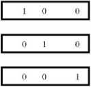
The data set was filtered, and maximum number of times of a course can be repeated for any single student was found to be 3; hence it was inferred that this prediction problem should have 3 classes. Each class represents the number of times a student repeats a course. Consequently, the designed networks should then have 3 neurons in the output layer; each neuron responding maximally to a particular class depending on the supplied input attributes. The full coding analogy is shown below.

• -    Student repeats course once

• -    Student repeats course twice

• -    Student repeats course thrice

Fig. 4. Output coding network classes

• IV. training and Testing of Networks

  The number of training samples that was used in this research is 4,000, hence considering the number of attributes for each input sample, the input training data matrix for the network is 30 × 4000; and the output target data matrix is 3 × 4000.

From the design perspective of neural networks, the dimensionality of the training data therefore necessitates that the number of input neurons is 30, and the number of output neurons be 3; the number of hidden neurons could not be determined be determined at this stage as it is generally obtained heuristically during the training phase of neural networks. For the purpose of cross-validation, 15% of the training data was used to perform 10-fold cross-validation in order to fight the network only memorizing (i.e. fight over-fitting). During training, errors on both the training data and validation are both monitored, and training was stopped once the error on the validation data began to rise for some consecutive epochs, even though the error on the training data may be decreasing still; this greatly improves the generalization power of the trained network.

For the purpose of testing the performance of the network, 1,500 samples were used, giving an input matrix of 30 × 1500, and an output target of 3 × 1500. The trained network is simulated with the test data, and the actual output classes compared against the target or desired output; hence, an important performance parameter of the trained network “recognition rate” can be evaluated using the equation given below. It is to be noted that the data used to test the networks were not part of the training data, as this discourages the trained networks from giving a performance based on memorized data, if the training data were used for testing. i.e. generalization power of trained networks can hence be better assessed.

no.of samples classified correctlyTotal number of test samples

Where, r.r is the recognition rate of the trained neural classifier.

• A.    BPNN

A single hidden layer back propagation network was trained with data as described above using different values for different parameters such as learning rate, momentum rate, maximum epochs, and the number of hidden neurons. Log-Sigmoid activation functions were used in the hidden and output layers. The training parameters for the network are shown in table 2.

Table 2. BPNN heuristic training

Network parameter	Value
Number of training samples	4,000
Number of hidden neurons	6
Learning rate (η)	0.2
Momentum rate (α)	0.9
Maximum epochs	2000
Training time (seconds)	143
Mean Square Error (MSE)	0.2138

Several experiments were performed, varying the number of hidden neurons, learning rate, and momentum rate. It can be seen in the table above that the after 2000 epochs, the back propagation network achieved an MSE of 0.2138, taking 143secs. 6 hidden neurons were found to give the best performance after several trials.

The added momentum rate added ensures that the network achieved a smooth learning curve, and therefore reduces rapid perturbations of the error being minimized during training; also, it reduces the possibility of the network getting stuck in a poor local minimum.

Below in fig.5 is shown the learning curve for the BPNN.

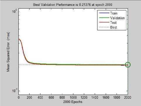
Fig. 5. MSE plot for BPNN training

The trained BPPN was tested by simulating with data that were not part of the training data, and the result is presented in the table below.

Table 3. Testing of BPNN

Network parameter	Value
Number of test samples	1,500
Correctly classified samples	1,294
Recognition rate	86.3%

The BPNN was tested with 1,500 samples, and a recognition rate of 86.3% was obtained.

• B.    RBFN

The heuristic training parameters for the RBFN network is shown below in table 4, Gaussians activation functions were used in the hidden layer, while linear activation functions were in the output layer of the network. The MSE plot for the network is shown in fig.6.

Table 4. Training of RBFN

Network parameter	Value
Number of training samples	4,000
Number of hidden neurons	8
Spread constant	1.0
Maximum epochs	875
Training time (seconds)	325
Mean Square Error (MSE)	0.0604

An MSE of 0.0604 was achieved after 875 epochs, with a training time of 325secs.

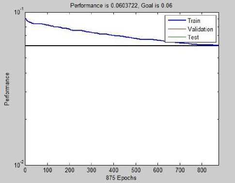
Fig. 6. MSE plot for RBFN training

The RBFN was also tested with the same 1,500 data samples as done with the BPNN, and the results presented in table 5.

Table 5. Testing of RBFN

Network parameter	Value
Number of test samples	1,500
Correctly classified samples	1,272
Recognition rate	84.8%

A recognition rate of 84.8% was obtained for the simulation of the RBFN.

• IV. Conclusion

The capability of neural networks to be applied in the knowledge discovery or mining of important relationships between some factors and corresponding effects have been exploited in this work. Furthermore, it is the believe that tools such as neural networks suffices in situations such has been presented in this work, the ability of academic administrators to exploit this approach in the prediction of students’ performance based on collected data is quite plausible. In addition, it is possible through such an approach as presented in this research to be able to fine-tune some of the critical factors (see section 3) considered to affect students’ performance, and hence re-simulating trained networks in order to evaluate how much the suggested changes in attributes or factors have effected a change in the students’ performance. This technique can allow the design or redesign of academic environments, study plans, and student-lecturer interrelation in such a way that improves overall students’ performance, which can be verified by a lower simulated number of students who will probably repeat a course twice or thrice, given the presented factors or attributes.

Future works include the optimization of this learning problem; genetic algorithms may be used to explore input attributes that are more significant than others, contributing more to the correct prediction of a student’s performance, and hence a better overall classification accuracy. Also, the use of multi-class support vector machine can be considered.