Decision-Making Using Efficient Confidence-Intervals with Meta-Analysis of Spatial Panel Data for Socioeconomic Development Project-Managers

Published Online August 2012 in MECS

Meta-analysis represents the statistical analysis of a collection of analytic results motivated by the gainful urge to integrate the findings in the context of geospatial data that represent environmental and socioeconomic indicators in a given context. This paper is in sequel to [8]. It is quite common to have access to panel data generated by a set of similar spatial data for analyses in a meta-data setup. Within this context, researchers often employ pooling methods to evaluate the efficacy of metadata analysis. One of the simplest techniques used to combine individual study results is the fixed-effects model, which assumes that a true effect is equal for all studies. An alternative, and intuitively more appealing method, is the random-effects model.

The purpose of this paper is to address the estimation problem of the fixed effects model and to present a simulation study of an efficient estimation of a mean true effect using panel data and a random effects model in order to establish appropriate ‘Confidence Interval’(CI) estimation for being readily usable in a decision-makers’ setup..

In that paper of [8], is attempted to be improved by proposing a method of statistical estimation aimed at improving the accuracy of the resultant CIs for an efficient estimation of a mean true effect using panel data and a random effects model. The improvement of the reliability, which has been demonstrated by the use of a simulation study, is two-fold namely mathematical statistically using the concept of the ‘Minimum Mean Square Estimator (MMSE)’ of the reciprocal of the heterogeneities [using the ‘Bootstrapping’] of the studies, and by computing the simulational averages and hence the “Relative Efficiency (REff.)’ of the estimator(s), using ’11,000’ replications in the simulation. Bootstrapping is the well-known technique of ‘Data Mining’ [Please peruse the relevant details in ‘APPENDIX # 2’ in this paper].

To illustrate the universal applicability of the impugned technique of ‘Meta-Analysis of the PanelData’ targeted in this paper in the areas additional to that of the socio-economic studies, as well-illustrated in the [8]’s paper, we take the example of the currently important ‘Global Warming Problem & Environmental Pollution’. For the ‘Decision-Making Managers’ at United Nation, we could construct the handy CIs (Confidence-Intervals) for their decision-making and the judgment regarding the allocations of the combating-resources to fight-down the awe-fully significant environmental-pollution-threat to humanity, including the moneys to the various countries/ continents on the earth, we would do well to make good use of the ‘Geospatial Panel Data’. The Meta-Analysis would have to be carried up in a hierarchical-setup. The Overall Global CIs would also be available finally to the decision-manager @ UN consequent upon this hierarchally carried out meta-analysis. The Final Global Meta-Analysis could have been using the ‘Continental Geospatial Data’; The Continental Meta-Analysis could have, well, been using the data for various countries in the continent; The Country-wise Meta-Analysis could well be using the Meta-Data of various states in the country, and finally the state-wise Meta-Analysis would have to be using the Geospatial Meta-Data of the various cities and the counties therein! At the grass-root level as well, we might well use the ‘Geo-Temporal Data’. For example, for the study of the ‘Environmental Pollution’ in a city by the harmful emissions from the automobiles commuting therein, the Data would vary temporally at the peak/ moderate/ less-busy hours of the day/ night, etc., etc! It would be in place to mention that the cases of missing/ poor data in underdeveloped/ developing countries in the aforesaid context could well be dealt-with by generating the relevant synthetic data to take care of such Geo-Spatial-Temporal Data Gaps through the use of well-known powerful statistical techniques.

Incidentally, such meta-analyses of ‘panel-data’ are gaining quick-currency amongst medical researchers, and are becoming increasingly popular day-by-day in their research investigations, where information on efficacy of a treatment is available from a number of clinical studies with similar treatment protocols. Often, when one study is considered separately, the data therein (as generated per the randomized control clinical trial(s)) would be rather too small or too limited in its scope to lead to unequivocal or generalizable conclusions concerning, for example, the effect of the socio-economic co-variates under investigation, in the target study of the predecessor-paper.

A number of methods are available to set up the confidence limits for the overall mean effect(s) for the meta-analysis of the panel-data in the context of a random/fixed effects model generated by these data on the socio-economic variable(s). A popular and simple commonly-used method is the one proposed by the [4] approach. It is worth noting, in the context of panel data/ meta-analysis, that the simplest statistical technique for combining the individual study results is based on a fixed effects model. In the fixed effects model, it is assumed that the true effect is the same for all studies generating the panel data. On the other hand, a random effects model allows for the variation in the true-effect across these studies in various states (in a federal setup like in U.S.A./India, e.g.)/ districts/ Counties/ municipalities/village panchayat/block therein, and is, therefore, more realistic a model.[5], in a systematic search of the first ten issues published in 1982 of each of the four weekly journals (NEJM, JAMA, BMJ, and Lancet) found only one article (out of 589) that considered combining results using formal statistical methods. The basic difficulty one faces in trying to combine/integrate the results from various studies is generated by the diversity amongst these studies at hand in terms of the methods employed therein as also the design of these studies Also due to different parent populations and varying sample sizes, each study has a different level of sampling error. Hence, while integrating the results from such varied studies, one ought to assign varying weights to the information stemming from respective studies; these weights reflecting the relative ‘value’ of each of this information. In this context, [1] highlighted the need for the careful considerations in developing the methods for drawing inferences from such heterogeneous, though logically related, studies. [2] Observed that, in this setting, it would be more appropriate to use a regression analysis  to characterize the differences in study outcomes.

In the context of a random effects model for the meta/panel-data analysis, there are a number of methods available to construct the confidence limits for the overall mean effects. [9] Proposed a simple confidence interval for meta-analysis, based on the t-distribution. Their approach, as per the simulation study, is quite likely to improve the coverage probability of the [4]’s approach. In the present paper we propose a couple of more efficient constructions of this confidence interval. A simulation study is carried out to demonstrate that our propositions improve the coverage probability of both of the aforesaid methods.

• 1.1    Geo-spatial Mapping

Mapping of spatial data has been investigated in many contexts. Lately though, access to mapping technology and geo-spatial software has given rise to applications called mashups (). In a mashup application, the mapping engine is provided by an independent service provider, and the spatial data typically comes from an independent source. The geo-spatial data is layered over an existing mapping structure to provide a composite map.

One example of such an application in the US context is Housing Maps (). This mashup application utilizes Google, Inc.'s mapping technology by accessing its published Application Programming Interfaces (API). Via this API, Housing Maps passes street-level address coordinates and related information (housing prices in this case) to the Google service, thereby creating a housing map. The data for housing comes from yet another freely-accessible service called Craigslist. This service allows interested landlords to post their real estate properties for rent or sale. The owner posts a location, price and description. Craigslist service then makes this information available via their website. As is evident from the following figure, the housing data is "mashed up" with the mapping service to create a composite application for geo-spatial representation of real estate in a given geographical locality (in this case, San Francisco, CA).

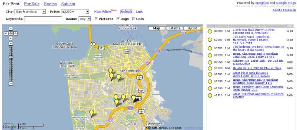
Fig. 1: JPDA algorithm flow chart

Data collected for many socio-economic or healthcare projects are often incomplete or inconsistent due to several issues such as data collection errors, social taboo or illiteracy reasons. Data collected from multiple sources can compound the problem, especially when we layer different data sources over a common geo-spatial space. Better estimators are needed for assessing the representation of data particularly in cases where the point estimation holds little meaning and an interval provides more latitude for interpretation.

In the next section, we will look at a particular project and its data collection efforts.

• 1.2    B.E-immunization

This project is a relatively new approach for immunizing children against fatal childhood diseases in Khammam District in Andhra Pradesh. It has helped in bringing immunizations closer to the communities scattered in the hard-to-reach areas. The project's aim is to increase the reach of immunization in developing countries with the help of Information and Communication Technology. Health workers capture details on a handheld device at the point of immunization. After giving the shot to a baby, the health worker updates the shot history. A receipt is also generated for the parents.

The project was initiated by Rajendra Nimje, a research fellow at Stanford University. From a news item on the project: Khammam Collector Rajendra Narendra Nimje, who was a "digital vision fellow'' of Stanford University during 2003-2004, had undertaken the project as part of his fellowship. The prototype of the concept was developed and tested in Nalgonda district from December 2003 to April 2004. Egged on by the success, the e-immunization was taken up in select villages. People of Edullacehruvu, Ramana Tanda, Bisarajapalli Tanda, Balajinagar Tanda, Balam Tanda under the Tirumalayapalem sub centre and Erragadda, Kokkireni, Tallacheruvu, Gopalapuram, Timmakkapeta villages under Kokkireni sub centers were the first in the district to enjoy the benefits of the e-immunization programme launched about a year ago (on March 9, 2005).

This project is a prime example of data being generated on the field by trained and untrained individuals. In this case, a certain degree of automation will help in reducing errors during data collection. Data from this project can be combined with census data from the same district and be mapped on a geo-spatial platform, thereby providing us with an immunization density map of the district of Khammam. The mapping of such data will provide with interesting insights, but point estimates are not very meaningful in this context. A better estimator of such efforts would be an interval estimate. We address this problem in the next sections.

• II.    The Problem Formulation

The statistical inference problem is concerned with using the information from ‘k’ independent studies in the meta-analyses setup. Set the random variable ‘yi’ to stand for the effect size estimate from the ‘ith.’ study. It would be in order to note here that, some commonly used, measures of effect size are mean difference, standardized mean difference, risk difference, relative risk, and odds-ratio. As the ‘Odds-Ratio (OR)’, which is of particular use in retrospective or case-control studies, is mostly used, we would confine to it for the simplicity of illustration in our paper. Nevertheless, it is without any loss of generality inasmuch as the details of this paper are analogously valid for the other measures of effect size.

Let nti and nci denote the sample sizes and let pti and pci denote the proportions dying (not achieving the stipulated goal) for each of the treatment (t) and control (c) groups, where ‘i’ stands for the designation of the study number: ‘I = 1 (1) n’. Also, let xti and xci denote the observed number of the deaths for the treatment and the control groups respectively, for the study number ‘i’. We note that for the ‘ith.’ study the following gives the observed log-odds ratio (log (ORi)) and the corresponding estimated variance.

_{ORi =} (1 - pci).pti _, p_ci.(1 - p_ti)

₂    ∧ ₂

estimated(σi)2 ≡ (σi)2 = = estimated (var(log(OR i))) =    +           +    + xti (nti -xti)   xci   (nci -xci)

The important point to be noted at this stage is that the estimated ( σ )² is rather a very close estimate of the respective population variance ( _σ )² , and that it is analogously closely available for the population variances for the cases of other measures of the effect size. For example, if the effect size y i happens to be the difference in proportions, ‘p_ti - p_ci‘, we estimate the population variance ( σ _i)² by:

₂    ∧ ₂

Estimated( σ _i)   ≡ ( σ i)   = p_ti(1 - p_ti)/p_Ci(1 - p_Ci).

Now, we might note that the general model is specified as follows.

y_i =θ _i +ε _i,i = 1,...,k; Wherein,

ε _i ≈ N(0, σ _i²) ;

And,

θ _i =µ+∂ _i; Wherein,

∂ i ≈ N(0, τ ²) .

Hence, essentially the model comes to be: y_i = µ+∂ _i +ε _i;i = 1,..., k

It is also important to note that whereas _∂ stands for the random error across the studies, ε represents the random error within a study, and that _∂ and ε are assumed to be independent. Also, the parameter τ ² is a measure of the heterogeneity between the ‘k’ studies. We will refer to it in our paper as the ‘heterogeneity variance’, which it is often called by.

Perhaps the important and the most crucial element in the panel-data/meta analysis is the challenge of developing an efficient estimator of this heterogeneity variance’ τ ²’. [4] Proposed and used the following estimate:

Estimate of (τ2) = max{0,

∑ _i ^k _{= 1}wi(yi -µ ^∧ )² - (k - 1)

^∑ i^k = 1^wi ^-∑ i^k = 1^wi^{2/ ∑} i^k = 1^wi

Wherein, w =1/σ2 and the weighted estimate of the ii mean effect is given by:

^{∧ µ=∑} i^k = 1^{wiyi/ ∑} i^k = 1^wi

Also, herein the weight ‘w i ’ is assumed to be known.

Earlier, we noted that the estimated ( σ i )² is rather a very close estimate of the respective population variance ( σ i )². Therefore, most usually the sample estimate ( ^∧ _σ )² is used in place of ( σ _i)², so that w_i = 1/( σ _i)² is used in (1), and estimated w i , i.e. _w ^∧ _{= 1/} ( ^∧ _σ )² in (2).

Recently, [9] proposed a simple confidence interval for the meta-analysis. This approach, consisting in the construction of the confidence interval based on the‘t-distribution’, significantly improved the ‘coverage probability’ compared to the existing ‘most popular’ [4]’ s approach, as outlined above.

It is worth noting, in the above context, that recently [3] presented a comprehensive summary of the existing methods of constructing the confidence interval for meta-analysis and carried out their comparisons in terms of their ‘coverage probabilities’.

While, the most-commonly-used/popular method of [4] random effects method led to the coverage probabilities below nominal level, the profile likelihood interval of [6] led to the higher coverage probabilities.

However, the profile likelihood approach happens to be quite cumbersome computationally, and involves an iterative calculation as does the ‘simple likelihood method’ presented in [3]. On the other hand, [3]’ s proposition of a simple approach for the construction of a ‘100(1-α)’ percent confidence interval for the overall effect in the random effects model, suing the pivotal inference based on the t-distribution, uses no iterative computation like the popular method of [4].

Moreover, the [9]’ s proposition has a better ‘coverage probability’ than that of [4]. Consequently, while [4]’ s confidence interval for meta-analysis used to be the most popular/commonly-used confidence interval, that of [9]’ s happens to be rather-the-best one in terms of the most important count, namely that of the ‘coverage probability’, on which the ‘confidence intervals’ are compared and rated.

In fact, therefore, our motivation is basically to attempt the improvement of these two methods for constructing the ‘Confidence Intervals’ for an interval estimate for the overall mean effect across the ‘k’ studies, using the panel/meta-data generated by these studies. The impugned improvement was targeted mainly at the improved ‘coverage probabilities’. It is amply achieved, as is revealed by the comparison using a ‘Simulation Study’. The modified “[9] Estimator (MSJE)” proposed in this paper turns up to be the best to use.

• III.    The Proposed Confidence Interval Estimates

As noted in the last section, the important and the most crucial element in the panel-data/meta analysis is the challenge of developing an efficient estimator of this heterogeneity variance’ ^{τ 2} ’. [4]’ s approximate 100(1-α) per cent confidence interval for the general mean effect ‘μ’, using the random effects model, is given by:

µ+ / - z _{α /2}(1/ ∑ _i ^k _{= 1}w_i)

∧∧  ∧

Wherein, µ = ∑ _i ^k _{= 1}wi y_i / ∑ _i ^k _{= 1}wi

∧  ∧∧

Also, wi = 1/(( σ i) + ( τ ) ) is evaluated using:

∧ ₂           ∑ ^k wi(yi -µ ^∧ )² - (k - 1)

( τ )   = max{0,    ^{i = 1}                         } , as in (1)

^∑ i^k = 1^{wi -∑} i^k = 1^wi^{2/ ∑} i^k = 1^wi

It would be in order here to note that zα/2 in (3) above is the α/2 upper quantile of the standard normal variable. To construct an alternative simple confidence interval for the general mean effect ‘μ’, using the random effects model, assuming that yi ≅ N(µ, (σi)2 +(τ)2)

Recently Sidik and Jonkman (2002) proposed an improvement. They, subject to the assumption that ∧∧ wi = 1/(σi)2 ’s correct weights ((i.e., essentially

∧ that wi ≈ wi ∀i = 1,2,...k. ), being close estimates), noted that:

Zw

^∧ /

( µ-µ )  (1/ ( ∑ _i ^k _{= 1}

∧ wi)) ≅N(0,1)

and k∧     ∧

Q_w = ∑ wi(y_i -µ )² ≅ χ ₍ ² _k

They showed that Zw and Qw are independently distributed. Hence, it follows that:

∧

( µ- µ ) ( ∑_i ^k _{= 1}

∧ ^wi⁾

^{≅ t}(k - 1)

k ∧      ∧

∑ wi(yi - µ )²/(k - 1)}

This, thence, led to [9]’ s proposition of an approximate 100(1-α) per cent confidence interval for the general mean effect ‘μ’, using the random effects model, is given by:

∧

^{µ+ / - t}k - 1, α /2

{

∧

^∑ i^k = 1^wi(yi

∧ µ )

∧ (k - 1) ∑ _i ^k _{= 1}wi

}

As noted earlier, under the  assumptions that

∧∧ wi = 1/(σi)2 ’s correct weights  ((i.e., essentially

∧ thatwi ≈ wi ∀i = 1,2,...k. ), being close estimates) and that ∂i and εi are independent (all assumptions being well-known to be quite reasonably tenable), we have (to the extent of the approximation due to the extent of the tenability of the aforesaid assumptions):

It would be in order here to note that tk-1, α/2, in (6) above, is the α/2 upper quantile of the t-distribution with k-1 degrees of freedom. Also, under the assumption of known weights,

Q_w/ [ (k _- 1) ∑ k _w ^∧ ] is an unbiased estimator of

∧ the variance of µ

It is very significant fact at this stage to note that both [4]’ s, as also [9]’ s 100(1-α) per cent confidence interval for the general mean effect ‘μ’, using the random effects model, are ‘approximate’, inasmuch as their validity is subject to the extent of the truth of the underlying assumption that the weights:

∧ wi ≈ wi ∀i = 1,2,...k. ,

∧ and hence the (σi)2 ≈ (σi)2,∀i = 1,2,...k.

Thus, essentially, it boils down to as to how efficient our estimate of the inter-study heterogeneity variance’ τ ²’ is. We might as well note here that:

If the estimate of (τ2), i.e. ∧ 2   , the random effects model boils down to the fixed-affect model.

Further, we might mention here that the more efficient estimation of the inter-study heterogeneity variance’ τ ²’ is the key motivating factor for our propositions to possibly improve the ‘coverage probability’. In both the papers, namely those of [4]a nd [9], the estimation of this inter-study heterogeneity variance’ τ ²’, as is nicely described in [3], is as follows:

The impugned two-stage random effects model:

yi = θ i + ε i,i = 1,..., k, Wherein, ε i ≈ N(0, σ i )

θ i = µ + ∂ i. Wherein ∂ _i ≈ N(0, τ ²) .

That could well be re-written equivalently as:

yi = µ+ ∂i +εi;i = 1,..., k ,  Wherein  εi ≈ N(0, σi )

and ∂ _i ≈ N(0, τ ²) .

k ∧

∑ wi( τ )y_i

µ ^∧ _τ = i = 1        ;

k ∧

∑ wi( τ )

i = 1

With variance:

∧ ₁

var( µ_τ ) =                             (8)

k ∧

∑ wi( τ )

i = 1

In the above,

∧ wi(τ) =[(wi) +(τ)2]

and

∧∧ wi =1/(σi)2; i=1, …, k(9)

Now, assuming that τ ² is known, we have:

∧

µτ ≅ N(µ,1) / ∑wi(τ))(10)

i = 1

It is interesting to note that the random effects model confidence intervals for μ are expected to be wider than those constructed under fixed effects model simply due to the facts that ∧ ≤ ∧ , and hence µ     µτ , var (µ∧) ≤ var (∧µτ ).

As τ ² is unknown in practice we ought to estimate it. [4] derived an estimate of τ ², using the meted of moments, by equating an estimate of the expected value of Q w with its observed value say, _{'q '} .

w

∧   ∑ ^k ( ^∧ w )²

E(Qw)=k-1+τ2(∑k wi-  1=1 i )= q∧ w             1=1           ∧      ∧ kw ∑1=1wi

Therefore, we note that if ‘t’is the solution of the above equation, we have:

[q ∧ - (k - 1)]

t =        ^w                              (11)

1 = 1             ∧

^∑ 1^k = 1^wi

So as to ward off the possibility of a negative value of‘t’ (which will be an unacceptable value of τ ², as any variance could not be negative), we define:

Estimated ( τ ²) = t if t >  0; and estimated ( τ ²) = 0

if t ≤ 0                                               (12)

Using (11) in (9), we get the w ^∧ _i( τ ) = [(w ^∧ _i) + ( ^∧ τ )²] ^{- 1} (wherein w ^∧ _i = 1/( ^∧ σ _i)² ); i=1, …, k to be used in (10), with the estimated variance of µ ^∧

∧∧ var(µτ)=                                    (13)

k∧

( ∑ wi( τ )) i = 1

Both, [4]’ s and [9]’ s propositions of an approximate 100(1-α) per cent confidence interval for the general mean effect ‘μ’, using the random effects model (as in (3) & (6), respectively), use the _µ ^∧ generated by the aforesaid and use the value of _v ^∧ _ar ( _µ ^∧ ) , as in (13).

Essentially our proposition of the improved Confidence Interval (CIs) estimates of the general mean effect ‘μ’ consist solely in a more efficient estimation of ’ _v ^∧ _ar ( _µ ^∧ ) ’ in (13). For this purpose the following results are importantly relevant:

Lemma: If an estimate, say ‘s²’ (usual unbiased sample variance estimator) of the population variance, say ‘ σ ²’ is based on a random sample X 1 , X 2 , … X k from a Normal population N (ө, σ ²), we have: {(k-1).s²}/ σ ² ≈ χ² (k-1) (: Chi-Square distribution on ‘(k – 1)’ degrees of freedom).

Further, we have: Minimum Mean Square Error Estimator MMSEE of ‘1/ σ ²‘is 1/ (k*.s²).

Wherein k* = (k-1)/ (k-5)                    (14)

Proof: As, in the case of the random sample from a normal distribution, it is rather very well-known that the ‘sample variance’ s² is a ‘complete sufficient statistic’ for the ‘population variance’ σ ². Therefore, Minimum Mean Square Error Estimator (MMSEE) of ‘1/ σ ²’ is simply its MMSE estimator of the class “M/ σ ²”.

Now, we use the following equations, which are easily derived:

E [(1/ s²)] = [(k-3)/ (k-1)]. (1/ σ ²)

E [(1/ s⁴)] = [(k-3). (k-5)/ (k-1)²]. (1/ σ ⁴).

Hence, we could easily establish that the Minimum Mean Square Error Estimator (MMSEE) of ‘1/ σ ²’ would be as stated in (14). Q. E. D.

Hence, we propose the following modified more efficient Cis, modifying the say, “Original DerSimonian-Laird Estimator (ODLE) [4]” , and modifying the say. “Original Sidik-Jonkman Estimator (OSJE) [9]” defined, respectively, in (3) and (6) above.

We would call our estimators as the “Modified DerSimonian-Laird Estimator (MDLE) [4]” , and as the “Modified Sidik-Jonkman Estimator (MSJE) [9]” , respectively.

Essentially, the ‘sole’ difference between ODLE & MDLE, as also between OSJE & MSJE consists in replacing ‘k’ in (3) and (6), respectively by ‘k* for the modifications under the TWO approaches consisting in “UMVUE’ estimation of ‘‘1/ σ ²‘, whereas ‘ σ ²‘ herein stands for the heterogeneity variance’ ^{τ 2} ’, and the parameter τ ² is essentially a measure of the heterogeneity between the ‘k’ studies.

• IV.    The Simulation Study

The format of the ‘Simulation Study’ in our paper to compare the “Original DerSimonian-Laird Estimator (ODLE) [4]” and the Original Sidik-Jonkman Estimator (OSJE) [9]” with our estimators “Modified DerSimonian-Laird Estimator (MDLE) [4], and as the “Modified Sidik-Jonkman Estimator (MSJE) [9]” , respectively, is the same as that in [9].

To compare the simple confidence interval based on the t-distribution with the DerSimonian and Laird interval in terms of coverage probability, we performed a simulation study of met analysis for the random effects model.

Throughout the study, the overall mean effect μ is fixed at 0.5 and the error probability of the confidence interval, α, is set at 0.05. We use only one value for μ because the t-distribution interval based on the pivotal quantity in (5) and the DerSimonian and Laird interval [4] are both invariant to a location shift. Three different values of τ ² are used: 0.05; 0.08, and 0.1. For each τ ², three different values of k (namely 10, 20, and 60 to keep the comparisons modestly) are considered. The number of simulation runs for the meta-analysis of k studies is 11 000. The simulation data for each run are generated in terms of the most popular measure of effect size in meta-analysis, the log of the odds ratio. That is, the generated effect size yi is interpreted as a log odds ratio (it could alternatively be the mean effect of the ith. Study, as well).

For given k, the within-study variance σi2 is generated using the method of [3]. Specifically, a value is generated from a chi-square distribution with one degree of freedom, which is then scaled by 1=4 and restricted to an interval between 0.009 and 0.6. This results in a bimodal distribution of σi2, with the modes at each end of the distribution. As noted by [3], values generated in this way are consistent with a typical distribution of σi2 for log odds ratios encountered in practice. For binary outcomes, the within-study variance decreases with increasing sample size, so large values of σi2 (close to 0:6) represent small trials included in the meta-analysis, and small values of σi2 represent large trials.

The effect size y i for i=1, …, k is generated from a normal distribution with mean μ and variance: σ _i² + τ ²

For each simulation of the meta-analysis, the confidence intervals based on the t-distribution and the [4] method are calculated, along with those of our proposed estimators “Modified Sidik-Jonkman Estimator (MSJE) [9]” are calculated along with those for “(Ordinary) Sidik-Jonkman Estimator (OSJE) [9]” . The numbers of intervals containing the true μ are recorded for all four methods. The proportion of intervals containing the true μ (out of the 11 000 runs) serves as the simulation estimate of the true coverage probability.

The results of the simulation study are presented in the tables (Nine Tables) in APPENDIX. From the tables, it can be seen that the coverage probabilities of the interval based on the t-distribution are larger than the coverage probabilities of the interval using the (Ordinary) DerSimonian and Laird method Estimator (ODLE) [4] for each τ ² and all values of k. Interestingly, our proposed estimator “Modified DerSimonian-Laird Estimator (MDLE) [4] performs even better than that. Although the coverage probabilities of the confidence interval from the t-distribution, like other methods, are below the nominal level of 95 per cent, they are higher than the commonly applied interval based on the [4] method, particularly when k is small. This suggests that the simple confidence interval based on the t-distribution is an improvement compared to the existing simple confidence interval based on [4] method. Incidentally, ‘MDLE’ is the best. The most remarkable fact is that our proposed estimator “Modified Sidik-Jonkman Estimator (MSJE) [9]” turns out to be the best in terms of the “Coverage Probability”!

• V.    Conclusion

As time is an important variable, and as Geospatial data would be temporal also, it is very significant to note that inasmuch as the ‘time’ could be viewed very conveniently in the shoes of ‘space’ the analogous treatment to ‘Geotemporal’ data in the meta-data set-up could well be carried out successfully, too! In fact the ‘Geo-Spatial-Temporal’ data in the meta-data setup dealt in two consecutive phases would be most realistic approach down-to-earth, as we have to carry out the analysis of ‘Geospatial’ data with this temporal toning-up to be realistic. This is the direction of our proposed future work in the area, and could well be the source of enthusiasm for other researchers, particularly in the meta-data set-up.