Decoding Optimization Algorithms for Convolutional Neural Networks in Time Series Regression Tasks

Convolutional Neural Networks (CNNs) have emerged as powerful models for various machine learning tasks, including image recognition, natural language processing, and time series analysis. In the domain of time series regression, CNNs have shown promising results in capturing temporal dependencies and extracting meaningful features from sequential data. However, the performance of a CNN model greatly depends on the optimization algorithm used during the training process.

Optimization algorithms play a critical role in updating the model parameters to minimize the loss function and improve the model's predictive accuracy. While numerous optimization algorithms have been proposed in the literature, their performance characteristics in the specific context of time series regression using CNNs have not been thoroughly explored.

The major research objectives of this study are twofold: first, to investigate the performance of various optimization algorithms in the context of time series regression using CNN models, and second, to evaluate their impact on the accuracy and convergence properties of the models. By conducting a comprehensive comparative analysis, we aim to provide insights into the suitability of different optimizers for time series regression tasks and identify their strengths and limitations.

While existing solutions employ optimization algorithms for training CNN models in various domains, their applicability to time series regression tasks using CNNs is not well understood. This research aims to address this gap by specifically focusing on the task of maximum temperature prediction using historical weather data. We will explore the performance of popular optimization algorithms such as Stochastic Gradient Descent (SGD), RMSProp, Adagrad, Adadelta, Adam, and Adamax in this specific context.

The main limitation of the existing research is the lack of comprehensive comparative analysis specifically tailored to time series regression using CNN models. By conducting a detailed evaluation of multiple optimization algorithms, we aim to fill this gap and provide researchers and practitioners with valuable insights for selecting the most suitable optimization algorithm for similar tasks.

The authors hope to achieve several outcomes with this research. Firstly, we aim to provide a comprehensive comparative analysis of optimization algorithms for time series regression using CNN models. Secondly, we aim to evaluate and compare the performance of different optimization algorithms based on various evaluation metrics, such as Mean Absolute Error (MAE), Mean Squared Error (MSE), Root Mean Squared Error (RMSE), R-squared (R²), Mean Absolute Percentage Error (MAPE), and Explained Variance Score (EVS). Finally, by analyzing learning curves, we aim to gain insights into the convergence behavior, speed, and stability of each optimizer.

The findings of this research will contribute to the existing knowledge by providing researchers and practitioners with a better understanding of the performance characteristics of different optimization algorithms in the domain of time series regression using CNN models. Ultimately, this research aims to assist in the selection of the most suitable optimization algorithm for accurate maximum temperature prediction, benefiting domains such as agriculture, energy management, urban planning, and others where temperature forecasting plays a crucial role.

The remainder of this paper is organized as follows: Section 2 provides an overview of related work on optimization algorithms in deep learning. Section 3 describes the dataset, and the methodology employed in this study is described in Section 4. Section 5 presents the experimental results and performance analysis. Finally, Section 6 concludes the findings of the work and outlines future research directions.

2.    Literature Review

Deep learning has emerged as a powerful paradigm for solving complex problems in various domains. LeCun et al. [1] provide a comprehensive overview of deep learning, highlighting its potential in transforming the field of machine learning. Goodfellow et al. [2] delve into the fundamental concepts of deep learning, presenting a comprehensive guide that covers both theory and practice. Convolutional neural networks (CNNs) have revolutionized image classification tasks. Krizhevsky et al. [3] introduced the influential AlexNet architecture, which achieved remarkable performance in the ImageNet challenge. The success of deep learning models like CNNs heavily relies on optimization algorithms.

One such algorithm is Adam, proposed by Kingma and Ba [4], which combines the benefits of adaptive learning rates and momentum. Zeiler [5] introduced ADADELTA, an adaptive learning rate method that does not require manual tuning. Tieleman and Hinton [6] presented RMSProp, which divides the gradient by a running average of its recent magnitude. These optimization algorithms have proven effective in training deep learning models.

Duchi et al. [7] proposed adaptive subgradient methods, which are particularly useful for online learning and stochastic optimization. Hwang et al. [8] conducted a comprehensive study on optimization algorithms for deep learning, exploring their impact on model training and convergence.

Time series forecasting is a crucial application area for deep learning. Bontempi et al. [9] discussed machine learning strategies specifically designed for time series forecasting. Deng and Yu [10] provided a comprehensive overview of deep learning methods and applications, including their relevance in time series analysis.

Gal and Ghahramani [11] introduced dropout as a Bayesian approximation, enabling deep learning models to represent model uncertainty. Graves [12] focused on generating sequences using recurrent neural networks (RNNs), which are effective for modelling time-dependent data. Lipton et al. [13] critically reviewed RNNs for sequence learning, highlighting their strengths and limitations.

Optimization algorithms play a crucial role in training deep learning models. Ruder [14] presented an overview of gradient descent optimization algorithms, including their variations and convergence properties. Srivastava et al. [15] proposed dropout as a simple yet effective regularization technique to prevent overfitting in neural networks.

Time series forecasting with deep learning has gained significant attention. Wang et al. [16] conducted a systematic literature review, exploring the use of deep learning for time series forecasting. Xu et al. [17] empirically evaluated the effectiveness of rectified activations in convolutional networks for time series analysis. Yao et al. [18] provided a comprehensive review of deep learning approaches for time series analysis, discussing their methodologies and applications.

In summary, the literature review highlights the significance of deep learning in various domains, including image classification and time series forecasting. It emphasizes the importance of optimization algorithms and explores their impact on model training. The use of deep learning for time series analysis, particularly in forecasting, has shown promising results, with various techniques and architectures being proposed and evaluated. The references provided serve as valuable sources to guide further research in this field.

3.    Data Description

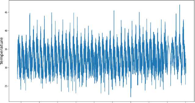
The dataset used in this research paper spans a period of 45 years, from January 1969 to January 2015, and focuses specifically on the daily maximum temperature recorded at Visakhapatnam airport. This dataset provides a comprehensive and long-term perspective on the temperature patterns and trends observed in the region. The dataset consists of daily measurements of the maximum temperature, capturing the highest temperature reached each day. These temperature values have been recorded consistently over the 45-year period, enabling a detailed analysis of the long-term temperature variations in Visakhapatnam.

Table 1. Temperature dataset

Date (DD-MM-YYYY)	Maximum Temp (°C)
01-01-1969	28.2
02-01-1969	28.8
03-01-1969	29.8
04-01-1969	30.6
05-01-1969	30.5
31-01-2015	30.4
01-02-2015	29.8
02-02-2015	28.8
03-02-2015	30.2
04-02-2015	32,4

By examining the daily maximum temperature data, researchers can gain valuable insights into the climate dynamics of the region. They can explore seasonal temperature variations, trends, and anomalies over the years, and investigate the influence of various factors, such as geographic location, elevation, or proximity to the coast, on temperature patterns.

Temperature Data

1970         1975         1980         1985         1990         1995         2000         2005         2010         2015

Date

Fig.1. Temperature dataset

The dataset serves as a valuable resource for climate research, climate modelling, and studies related to the impacts of temperature on various sectors such as agriculture, public health, and infrastructure planning. It provides a foundation for understanding the local temperature regime and its potential implications in the context of climate change.

The data collection process involved retrieving the historical temperature records, including the maximum temperature values, for the desired geographical region. The dataset includes relevant features such as date and time stamps, meteorological station identifiers, and additional environmental variables.

To ensure data quality, a series of data quality checks and preprocessing steps were performed. This involved handling missing values, identifying and addressing outliers, and verifying the consistency and reliability of the temperature measurements. Any inconsistencies or anomalies in the dataset were carefully addressed to maintain the integrity of the data. The dataset utilized for this piece of work has been sourced from India Meteorological Department.

4.    Methodology

This section outlines the methodology employed in the research paper to measure and compare the performance of different optimizers for time series regression using a convolutional neural network (CNN) model. The objective is to address the research objectives and provide a clear understanding of the experimental approach.

• 4.1.    The Optimizers

The research paper investigates the utilization of six distinct optimization algorithms: Stochastic Gradient Descent (SGD), RMSprop, Adagrad, Adadelta, Adam, and Adamax. These algorithms were chosen based on their wide adoption and success in deep learning, but their specific performance characteristics in the context of time series regression using CNNs have not been thoroughly explored. Each optimizer employs unique theoretical foundations and strategies to optimize the model parameters during the training process. The choice of these optimizers enables the investigation of their suitability for time series regression tasks, addressing the research objectives of evaluating their performance and impact on the accuracy and convergence properties of the CNN models.

Stochastic Gradient Descent (SGD) is a widely adopted optimization algorithm that aims to minimize the loss function iteratively. It achieves this by updating the model parameters using the gradients of the loss function computed on randomly selected subsets of the training data. SGD seeks to locate the global minimum of the loss function by gradually adjusting the parameters in the direction of the steepest descent.

RMSprop extends SGD by introducing an adaptive learning rate. It divides the gradient by the exponentially decaying average of the squared gradients. This approach enhances convergence speed and attenuates the influence of noisy gradients, leading to improved optimization performance.

Adagrad adapts the learning rate for each parameter based on the historical gradients accumulated over time. It assigns larger learning rates to infrequent parameters and smaller learning rates to frequent parameters. This adaptive learning rate scheme enables the algorithm to effectively converge in various directions within the parameter space.

Adadelta addresses some limitations of Adagrad by replacing the accumulation of past squared gradients with an exponentially decaying average. It also introduces a separate parameter to control the learning rate, enhancing stability, convergence, and eliminating the need for manual tuning.

Adam combines the concepts of momentum optimization and RMSprop. It maintains exponentially decaying averages of both the gradients and the squared gradients. By utilizing these first and second moments of the gradients, Adam achieves faster convergence and effectively handles sparse gradients.

Adamax is a variant of Adam that employs the infinity norm (maximum value) of the gradients instead of squared gradients. This modification enhances the algorithm's performance in scenarios involving large parameter updates.

By incorporating these optimization algorithms in the research paper, a comprehensive analysis and comparison has been conducted. The specific mathematical principles and heuristics employed by each optimizer enable efficient and effective updating of the model parameters during training. The examination of their performance using various evaluation metrics allows for an insightful assessment of their suitability for the specific task under investigation.

• 4.2.    Workflow

To ensure a comprehensive and rigorous analysis, a systematic workflow was followed throughout the research. The workflow consisted of several key steps aimed at addressing the research objectives and facilitating a fair comparison among the optimization algorithms.

The various stages employed in the workflow enable the achievement of the research objectives as follows:

• a)    Dataset Selection : The selection of a specific dataset suitable for time series regression ensures that the research is conducted on relevant data. The dataset is carefully sourced and preprocessed to ensure compatibility with the CNN model and the time series regression task.

The dataset selection was based on several valid reasons:

• •    Relevance to Time Series Regression : The dataset comprises a time series of historical temperature records, which aligns with the objective of time series regression analysis. By selecting a dataset with sequential data, the research can effectively evaluate the performance of different optimization algorithms in capturing temporal dependencies and predicting maximum temperatures accurately.

• •    Practical Significance : Accurate maximum temperature prediction has significant practical implications in various domains, including agriculture, energy management, and urban planning. By selecting a dataset

related to maximum temperature prediction, the research addresses a real-world problem and provides insights that can be directly applied in decision-making processes and planning activities.

• •    Availability and Quality : The dataset chosen for this research was carefully sourced and evaluated to ensure its availability and quality. It is essential to work with reliable and well-curated data to obtain meaningful research findings. The selected dataset meets these criteria, enabling robust analysis and reliable conclusions.

• •    Comparability and Reproducibility : The use of a specific dataset allows for comparability and reproducibility of the research findings. By employing the same dataset across different optimization algorithms, the methodology ensures a fair comparison, enabling researchers and practitioners to evaluate and replicate the results using the same dataset.

By considering these reasons, the selected dataset provides a suitable foundation for the research, aligning with the research objectives and facilitating a meaningful analysis of different optimization algorithms in the context of time series regression for maximum temperature prediction.

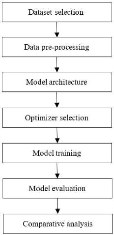
Fig.2. Model development workflow

• b)    Data Preprocessing : The preprocessing steps applied to the dataset handle missing values, outliers, or noise, which are common challenges in time series data. By addressing these preprocessing tasks, the methodology ensures that the input data is suitable for training and evaluating the CNN models, contributing to the accuracy and reliability of the results.

• c)    Model Architecture : The design of the CNN model specifically for time series regression considers the unique characteristics and requirements of this task. The selection of appropriate layers, hyperparameters, and activation functions ensures that the models can effectively capture temporal dependencies and extract meaningful features from the sequential data. This aspect of the methodology contributes to the accurate modeling of time series data.

• d)    Optimizer Selection : The evaluation of various optimization algorithms allows for a comprehensive analysis of their performance characteristics in the context of time series regression using CNN models. By comparing different optimizers, the methodology facilitates identifying the optimizer that yields the best performance, addressing the research objective of evaluating their impact on model accuracy and convergence properties.

• e)    Model Training : The iterative training process, conducted on the selected dataset using each optimizer, is crucial for optimizing the CNN models' parameters. By training the models over a fixed number of epochs and updating the parameters based on the optimization algorithms, the methodology enables the models to learn and adapt to the data, contributing to improved predictive accuracy.

• f)    Model Evaluation : The evaluation of the trained CNN models using various performance metrics, such as mean absolute error (MAE), mean squared error (MSE), root mean squared error (RMSE), coefficient of determination (R²), mean absolute percentage error (MAPE), and explained variance score (EVS), allows for a comprehensive assessment of their predictive performance. The methodology facilitates the comparison of the models' performance across different optimization algorithms, aiding in achieving the research objectives of evaluating their suitability for time series regression tasks.

• g)    Comparative Analysis: The comparison of the performance metrics obtained from the evaluation enables the identification of the optimizer that yields the best performance for the given time series regression task. This

• 4.3.    Model Evaluation

comparative analysis is crucial for understanding the strengths and limitations of each optimizer and contributes to the research objectives of evaluating their performance characteristics.

By following this methodology, the research aims to provide insights into the performance characteristics of different optimization algorithms in the context of time series regression using CNN models. The systematic workflow and the specific steps undertaken facilitate achieving the research objectives of evaluating the performance, impact, and suitability of the optimization algorithms for time series regression tasks. This methodology ensures a comprehensive and rigorous analysis, allowing for meaningful conclusions and recommendations to be drawn from the research findings.

Performance metrics play a crucial role in evaluating the effectiveness and accuracy of deep learning models. These metrics provide quantitative measures that allow us to assess the performance of different models, compare them, and make informed decisions. They provide objective measures to evaluate the performance of deep learning models. They enable us to assess accuracy, identify areas of improvement, compare models, and monitor progress.

The metrics used for the present piece of work are as follows:

• a)    Training loss : One of the primary evaluation metrics used is the training loss, which measures the model's ability to fit the training data. It is computed as the average loss over all training examples at each epoch of training.

• b)    Test loss : The test loss, on the other hand, measures how well the model can generalize to unseen data, and it is calculated as the average loss over all test examples.

• c)    Mean Absolute Error (MAE) : The MAE is a measure of the average magnitude of the errors in predictions and is computed as the mean of the absolute differences between the predicted values and the actual values.

The mathematical formula for Mean Absolute Error (MAE) is:

n

MAE = -£|y - У n1

where:

n: number of samples in the dataset

y: the actual value of the target variable ŷ: the predicted value of the target variable

• d)    Mean squared error (MSE) : The MSE measures the average squared difference between the predicted values and the actual values and gives higher weight to large errors than MAE.

The mathematical formula for Mean Squared Error (MSE) is:

n

MSE = - £ ( y - y ) 2

n 1

where:

n is the number of samples in the dataset y is the actual value ŷ is the predicted value

• e)    Root Mean Squared Error (RMSE) : RMSE, on the other hand, is the square root of the MSE and is more interpretable since it is in the same units as the target variable.

The mathematical formula for Mean Squared Error (MSE) is:

n

RMSE =

'^- z ( y - У ) 2 n 1

where:

n is the number of samples in the dataset y is the actual value ŷ is the predicted value

• f)    Coefficient of Determination (R²) : The R² score measures how well the model fits the data compared to a baseline model that always predicts the mean of the target variable, and it is a value between 0 and 1, with 1 indicating a perfect fit.

The mathematical formula for R² score (coefficient of determination) is:

^SS res

R 2 — 1--

SStot where SSres is the sum of squared residuals (or errors) and SStot is the total sum of squares, given by:

SS res

∑ (y true - y pred )2

SS tot =

∑ (y true – y mean

)2

ytrue represents the true values of the target variable, ypred represents the predicted values, and ymean represents the mean of the true values

• g)    Mean Average Percentage Error (MAPE) : MAPE, on the other hand, is a measure of the average percentage difference between the predicted values and the actual values, and it is computed as the mean of the absolute percentage differences.

The formula for MAPE is:

MAPE —

n

I

*

N

where:

n = number of observations

Σ = sum of the absolute percentage error for all observations y = actual value y ̂ = predicted value

• h)    Explained Variance Score : Finally, EVS measures the proportion of variance in the target variable that is explained by the model and is a value between 0 and 1, with 1 indicating that the model explains all of the variance in the target variable.

The mathematical formula for Explained Variance Score (EVS) is:

^V ar ⁽ У_№ - У рг^а ) EVS —------------

Var ( y_true )

where:

ytrue: the true target values ypred: the predicted target values

Var(): the variance of the inputs (in this case, the difference between true and predicted values)

The methodology section provides a clear framework for conducting the research and evaluating the performance of different optimizers for time series regression using a CNN model. It establishes the necessary steps to ensure rigorous experimentation and allows for the comparison of results to draw meaningful conclusions.

5.    Results 5.1.    Evaluation Metrics

The tables 2-7 present the evaluation metrics for each optimization algorithm, including overall training loss, test loss, mean absolute error (MAE), mean squared error (MSE), root mean squared error (RMSE), R-squared score (R²), mean absolute percentage error (MAPE), and explained variance score. These metrics provide a comprehensive assessment of the performance of each optimizer in the time series regression task. Based on the evaluation metrics obtained for the different optimization algorithms, we can analyze the results as follows:

Table 2. Evaluation metrics for SGD

Metric	Experimental Value
Training loss	0.00933134090155363
Test Loss	0.010679766535758972
MAE	0.08125873639183628
MSE	0.010679763864482694
RMSE	0.10334294298346014
R² score	0.37557915374023354
MAPE	26.099948032988458
EVS	0.40939352477370683

Table 3. Evaluation metrics for rmsprop

Metric	Experimental Value
Training loss	0.007017516531050205
Test Loss	0.008068193681538105
MAE	0.06877866620133112
MSE	0.008068192954149192
RMSE	0.08982312037637744
R² score	0.5282716044901101
MAPE	27.12916148166389
EVS	0.5915947010174196

Table 4. Evaluation metrics for adagrad

Metric	Experimental Value
Training loss	0.006606485228985548
Test Loss	0.006591032259166241
MAE	0.060052006496649095
MSE	0.006591033653585886
RMSE	0.08118518124378295
R² score	0.6146376582926396
MAPE	28.420254707647945
EVS	0.6152247820897447

Table 5. Evaluation metrics for adadelta

Metric	Experimental Value
Training loss	0.006538707297295332
Test Loss	0.006664424668997526
MAE	0.0605897819918501
MSE	0.0066644252111285
RMSE	0.0816359308829666
R² score	0.6103466253587104
MAPE	28.205422741966892
EVS	0.6138038300152554

Table 6. Evaluation metrics for adam

Metric	Experimental Value
Training loss	0.005343522876501083
Test Loss	0.005248242989182472
MAE	0.05075210626726345
MSE	0.005248242473027826
RMSE	0.07244475462742507
R² score	0.6931475219894085
MAPE	30.714420212958515
EVS	0.6946548864900536

Table 7. Evaluation metrics for adam

Metric	Experimental Value
Training loss	0.005115372594445944
Test Loss	0.0050387331284582615
MAE	0.049109275276953496
MSE	0.005038732711529309
RMSE	0.07098403138403249
R² score	0.7053970683496663
MAPE	31.116555029049316
EVS	0.710525571135542

• a)    Overall Training Loss:

• •    The overall training loss measures the average loss during the training process and reflects the optimization and convergence of the models.

• •    Lower values indicate better optimization and model convergence.

• •    Among the evaluated optimizers, Adamax achieved the lowest training loss (0.005115), followed by Adam (0.005344) and Adadelta (0.006539).

• •    Among the evaluated optimizers, Adamax achieved the lowest training loss, indicating its effectiveness in optimizing the model parameters and achieving convergence.

• b)    Test Loss:

• •    The test loss represents the model's performance on unseen data and reflects their generalization capability and prediction accuracy.

• •    Lower values indicate better generalization and prediction accuracy.

• •    Adamax achieved the lowest test loss (0.005039), followed closely by Adam (0.005248) and Adadelta

  (0.006664).

• •    Adamax achieved the lowest test loss, indicating its ability to generalize well to unseen data and make

accurate predictions.

• c)    Mean Absolute Error (MAE):

• •    MAE measures the average absolute difference between predicted and actual values and provides insights into the accuracy and precision of the models.

• •    Smaller MAE values indicate better accuracy and precision.

• •    Adamax achieved the lowest MAE (0.0491), followed by Adam (0.0508) and Adadelta (0.0606), indicating the ability of Adamax to minimize the prediction errors and achieve better accuracy.

• d)    Mean Squared Error (MSE) and Root Mean Squared Error (RMSE):

• •    MSE and RMSE quantify the average squared and square root of the difference between predicted and actual values, respectively, and provide information about the predictive accuracy of the models.

• •    Lower values indicate better predictive accuracy.

• •    Adamax achieved the lowest MSE (0.005039) and RMSE (0.070984), followed closely by Adam, indicating its ability to minimize the squared errors and improve the precision of predictions.

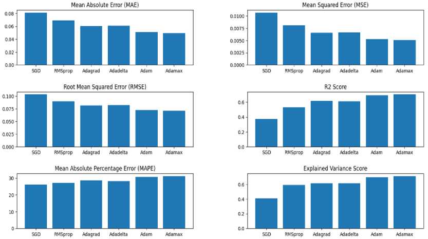
Fig.3. Evaluation metrics for different optimizers

• e)    R-squared Score (R²):

• •    R² measures the proportion of variance in the dependent variable that is explained by the model.

• •    Higher R² values indicate better model fit and prediction performance.

• •    Adamax achieved the highest R² score (0.705), followed by Adam (0.693) and Adadelta (0.610), indicating its

ability to capture and explain a larger proportion of the variance in the target variable.

• f)    Mean Absolute Percentage Error (MAPE):

• •    MAPE measures the average percentage difference between predicted and actual values and provides insights into the prediction accuracy of the models.

• •    Lower MAPE values indicate better prediction accuracy.

• •    Adamax achieved the lowest MAPE (31.12%), followed by Adam, indicating its ability to make predictions with lower percentage errors.

• g)    Explained Variance Score (EVS):

• •    EVS represents the proportion of variance in the dependent variable that is explained by the model and provides information about the prediction performance of the models.

• •    Higher values indicate better model fit and prediction performance.

• •    Adamax achieved the highest EVS (0.710), followed by Adam and Adadelta, indicating its ability to explain a larger proportion of the variance in the target variable.

• 5.2.    Analysis of Learning Curves

Based on these metrics, it can be observed that Adamax and Adam consistently performed well across multiple evaluation criteria, including training loss, test loss, MAE, MSE, RMSE, R², MAPE, and EVS. Adadelta also showed competitive performance, particularly in terms of R² and EVS. These findings suggest that Adamax, Adam, and Adadelta are effective optimization algorithms for the time series regression task, showcasing their ability to optimize the model and yield accurate predictions.

The variation of training loss with batches and the test loss is plotted graphically in Fig 1. The learning curves provide valuable insights into the convergence behaviour of the optimizers during the training process. By analysing the learning curves, we can observe how the loss changes over time and gain a better understanding of how each optimizer performs in terms of convergence and model improvement. Upon analyzing the learning curves for the different optimizers, the following observations can be made:

SGD : The learning curve analysis reveals that the SGD optimizer demonstrates a gradual convergence of the model over the training iterations. The training loss consistently decreases with each iteration, indicating that the model is learning and improving over time. The loss reaches a value of 0.0093, suggesting that the model's performance improves as the training progresses.

RMSProp: The learning curve analysis for RMSProp shows a similar pattern to SGD, with a consistent decrease in the training loss. However, the rate of decrease is slightly faster compared to SGD, indicating a relatively better convergence. The loss converges to a value of 0.00701, which suggests that the RMSProp optimizer helps the model achieve improved performance compared to SGD.

Adagrad : The learning curve analysis reveals that Adagrad exhibits a slower convergence compared to both SGD and RMSProp. The training loss steadily decreases but at a slower pace. The loss reaches a value of 0.0066, indicating a relatively slower convergence compared to the other optimizers. This suggests that Adagrad may require more iterations to reach optimal performance.

Adadelta : The learning curve analysis for Adadelta demonstrates a similar pattern to Adagrad, with a gradual decrease in the training loss. However, the rate of decrease is slower compared to RMSProp. The loss converges to a value of 0.0065, indicating a relatively slower convergence similar to Adagrad. This suggests that Adadelta may require more training iterations to achieve optimal performance.

Adam : The learning curve analysis reveals that the Adam optimizer exhibits a rapid decrease in the training loss during the initial iterations, followed by a slower rate of decrease. The loss reaches a value of 0.0053, indicating a relatively faster convergence compared to the other optimizers. This suggests that Adam is effective in quickly improving the model's performance.

Adamax : The learning curve analysis for Adamax shows a similar pattern to Adam, with a rapid initial decrease in the training loss followed by a slower rate of decrease. The loss converges to a value of 0.0051, indicating a relatively faster convergence similar to Adam. This suggests that Adamax performs well in terms of convergence speed.

Overall, it can be observed that Adam and Adamax demonstrate faster convergence compared to the other optimizers, while Adagrad and Adadelta exhibit relatively slower convergence. RMSprop falls in between, showing a moderate convergence rate. These optimizers exhibit quicker learning, achieve lower loss values, and effectively capture the underlying patterns in the time series data. The learning curves provide valuable insights into the convergence behavior of the optimizers and help in understanding their impact on the performance of deep learning models.

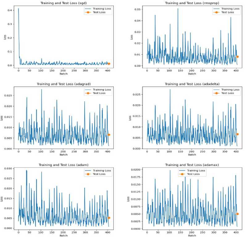
Fig.4. Learning curves for different optimizers

• 5.3.    Discussion

6.    Conclusions

The evaluation metrics provide valuable insights into the performance of different optimization algorithms for time series regression using CNN models. The results indicate that Adamax, Adam, and Adadelta are effective optimization algorithms for this task, as they consistently demonstrate better performance across multiple evaluation criteria.

The learning curves analysis further supports these findings. Adamax and Adam exhibit faster convergence compared to the other optimizers, while Adagrad and Adadelta show relatively slower convergence. The learning curves illustrate the improvement of the models over the training iterations and provide a better understanding of the convergence behavior of the optimizers. Overall, the results demonstrate the importance of selecting an appropriate optimization algorithm for time series regression tasks using CNN models. The findings suggest that Adamax, Adam, and Adadelta are well-suited for this task, as they consistently achieve better performance in terms of accuracy, precision, generalization, and model fit.

In this research paper, we conducted a comprehensive analysis to compare the performance of different optimization algorithms in time series regression tasks using CNN model. The evaluation metrics including overall training loss, test loss, mean absolute error (MAE), mean squared error (MSE), root mean squared error (RMSE), R-squared score (R²), mean absolute percentage error (MAPE), and explained variance score were used to assess the performance of each optimizer. Based on the experimental results, it is evident that the choice of optimization algorithm significantly impacts the performance of deep learning models in time series regression. Among the evaluated optimizers, Adam and Adamax consistently demonstrated superior performance across various metrics. These algorithms consistently achieved lower training and test losses, smaller MAE and MSE values, and higher R² scores, indicating their ability to accurately capture the underlying patterns in the time series data. Though they exhibited relatively higher MAPE values but the higher explained variance scores affirmed their effectiveness in predicting time series values. RMSProp, Adagrad, and Adadelta also showed competitive performance, although slightly inferior to Adam and Adamax. These optimizers demonstrated relatively higher losses and lower scores, but still performed reasonably well in terms of prediction accuracy and capturing the variance in the target variable. On the other hand, the Stochastic Gradient Descent (SGD) optimizer displayed relatively poorer performance compared to the other algorithms. It exhibited higher overall training and test losses, as well as larger MAE values, indicating challenges in effectively converging on the time series regression task. These findings highlight the importance of selecting an appropriate optimization algorithm when designing deep learning models for time series regression. Adam and Adamax are recommended choices due to their consistently strong performance across multiple evaluation metrics. However, the specific choice of optimizer should also consider the characteristics of the dataset and the specific requirements of the task at hand. Overall, this research contributes to the understanding of the impact of optimization algorithms on the performance of CNN model for time series regression. It provides valuable insights for practitioners and researchers in selecting the most suitable optimizer for their time series forecasting and prediction tasks. The scientific justification for this work lies in the practical importance of accurate time series regression models in domains such as finance, weather prediction, and resource planning. By identifying the most suitable optimization algorithms, researchers and practitioners can enhance the accuracy and reliability of their models, leading to better decision-making and forecasting. Future research can build upon this work by exploring additional optimization algorithms or hybrid approaches to further improve the performance and efficiency of deep learning models in time series regression. Additionally, extensions of this research could involve investigating the impact of optimization algorithms on different types of time series data or exploring the combination of optimization algorithms with other techniques to achieve even better performance. This research advances the field by providing insights into the impact of optimization algorithms on deep learning models for time series regression. It offers a scientific justification for the importance of selecting appropriate optimizers and suggests practical applications in various domains. By leveraging the findings of this research, researchers and practitioners can enhance the accuracy and reliability of their time series regression models, thus contributing to advancements in decision-making, forecasting, and planning.