Deep Learning based Real Time Radio Signal Modulation Classification and Visualization

Modulation classification is an inter modulation technique that determines modulation classes of incoming signals. Traditional AMC extracts information based on specialized training. Extraction of radio features are difficult and time consuming. Accuracy is strongly reliant on the radio characteristics that were extracted.

Automatic Modulation Classification helps to find the various categories of modulation in the received signals. The accuracy of classification in such categories is very much significant in defence applications, and in all other signals nature applications. Although various techniques are exist for signal modulation classification, the latest technique such as deep learning is playing important role in improving the accuracy of classification.

Deep learning is a machine technique that learns from large amount of data which is useful to solve complex problems though the dataset which is large. Deep learning models can be trained by using a set of data that learn features from data which eliminates the manual feature extraction.

The Deep Learning based Classification can extract the radio features and can also perform classification. Hence if the input is radio signal it can automatically learn features and can improve classification accuracy. Deep Learning based classifiers have been implemented in many of the fields like image classification, speech recognition and text classification. Though deep learning models are used in radio modulation it is still unclear and visualization is not used in radio modulation. Hence we will see about the visualization techniques used in radio modulation.

Here we can see Convolution Neural Network (CNN) and Long Short-Term Memory (LSTM)-based modulation classifiers from which we can classify and visualize radio signals. The CNN in deep learning is commonly applied for classification which uses a special function called as convolution. The CNN architecture contains convolutional layers, pooling layers and fully connected layers. During convolution the kernel moves along the input matrix and it generates the feature map, which is then given as input to next layer. The LSTM is a recurrent neural network which has been used in hand writing recognition, speech recognition and in predictions based on time data. The LSTM consists of three gates forget gate, input gate and the output gate which is used for predictions.

We evaluate these models on an open dataset RadioML2016. The dataset has modulated I and Q values of different modulation categories with different signal to noise ratio. Each modulation type contains 1000 modulated samples with length of 128. Here we will implement the visualization of the radio signals by introducing the class activation vector. We will introduce the activation threshold for visualizing the radio features by connecting the simultaneous sample points which are greater than the threshold.

We visualize both the CNN based classifier and LSTM based classifier, which will be extracting the same radio features of the radio signal. In CNN based modulation classifier we are using two types i.e., LeNet based classifier and ResNet based classifier which can be used to classify the radio signals. The LeNet consists of two convolutional layers and three fully connected layers. The ResNet consists of three residual stacks and three fully connected layers whereas the residual stack consists of five convolutional layers and one max pooling layer. The residual stack is followed by max pooling layer. In LSTM the features are similar to the knowledge of human experts. Both the LeNet and ResNet based classifier uses the in-phase and quadrature-phase signals as the input. The LSTM based classifier uses the amplitude and phase information as the input.

We will also be evaluating the radio signals with fewer sample points through the CNN based modulation classifier, ResNet based classifier to show that the classifier depends on the information carried by radio signal sample and if a radio sample of the length of 64 is given it may lead to misclassification.

2.    Literature Survey

Deep learning classifier has been successfully applied in classifying the radio modulation types, In [1], deep learning model it consist of multiple processing layers to representation of data with several level of abstraction. These are mostly used in speech recognition, object detection and visual object recognition. In [2] Automatic Modulation Classification uses statistical moments of signals which used to develop and classify the modulation types. It shows that nth statistical moment of the signal is monotonic increasing of Mth function. In [3], the cumulants based classification is high effective when it uses hierarchical modulation. Based on the element fourth order cumulants it proposes the hierarchical digital modulation. In [4], proposed Blind Modulation Classification which EC and cyclic cumulants are integrated in this technique. The EC is used to determine whether or not the constellations are real. The cyclic cumulants which will classify itself within the subclasses. The proposed modulation classification is used find the probability error in the classification.

In [5], the model for Automatic Modulation Classification (AMC) is defined based on long short term memory (LSTM) is proposed. The model learn time domain features and phase information of the data for modulation classification.The proposed model gives classification accuracy of 90% with varying signal to noise ratio. The LSTM model can learn good time domain representation which used to classify the modulation signals. In [6] the experimental results show when SNR is low, the suggested GCN algorithm provides higher accuracy than the CNN method. GCN cannot be directly used to perform modulation recognition since modulated signals are not graphs.In [7], the deep learning is predicted on large quantity of records for classification. In Deep learning there is no need to perform feature selections, which is easy to perform classification rather than any other machine learning models. In [8] proposed LeNet which uses in phase (I) and quadrature phase (Q) as a input and LeNet based modulation classifier outperforms expert features based algorithm for signal with low SNR value. In [9] proposed ResNet which further improve the performance by using amplitude and phase as a input.

In[10] Deep learning based Modulation classifier using data Augmentation is proposed which training deep learning model requires large amount of data, if data is not sufficient it will cause the overfitting of data. So we have to expand the dataset into large amount to overcome the over fitting problem hence the model performs well. In [11], the proposed the combination of inceptionResnetve2 and transfer adaptation. Constellation diagram has given input for the inceptionResnetv2 which identify different kind of signals. Transfer adaptation is used for feature extraction.SVM model is used to identify the modulation types.

3.    Methodology

A radio signal x of length N is belonging to one of the modulation categories, which is denoted by у of length N_y . In radio modulation classification we perform a mapping function which maps x^y to a vector у = [у_;- E (0,1) | j E N_y), where у_; denotes the probability of radio signal x to which modulation category it belongs.Now the predicted modulation category is taken by the greatest probability of у_; which is represented as j* = arg ma.X j _ENyy j .

For the deep learning based models we use the radio signals as input which is in the form of in-phase (I) and quadrature-phase (Q) samples, which is denoted as x_t = (I t , Q_t). This can also be transformed into amplitude (A) and phase (0) as x_t = (A_t, 0_t). This transformation can be done by using the formula,

A t = ^I 2 +Q

0_t = arctan(Q_t/I_t)

Modulation analyzers based on deep learning RadioML2016.10a is an open dataset that we used. The information contained in the dataset are modulated (I, Q) values under ten modulation categories of radio signals with different signal to noise ratio. Eight different modulation types are present in our RadioMl2016.10a dataset, they are 16QAM (quadrature amplitude modulation), 64QAM, GFSK, CPFSK, BPSK (binary phase shift keying), QPSK, 8PSK (phase shift keying), and PAM4 along with two analog modulation categories AM-DSB and WB-FM. Each of the modulation categories contains thousand signal samples of length 128 for each varying SNR. Here we use only the signals of SNR range from 0 db to 18 db to implement the CNN and LSTM based classifier.

We visualize by using a class activation vector w = {w_t E [0,1]|i E N^ where each w_t shows the significance of input x_t. For further visualization we plot a constellation diagram of radio sample x. Here each constellation point represents the radio sample x_t is either plotted by using I and Q values or by using the A and 0 values. Now we colour the point x_t ranging from yellow to red corresponding to the weight w_t. A point which has a greater weight has to be its highlighted in red since it's crucial for classification. We utilise an activation threshold ??_wand a time domain feature to show it.we have to connect each pair of two consecutive radio samples x_t and x_t+1 through a green line when both the points has a weight greater than threshold.

• A.    Visualizing CNN Classifier

A deep learning based CNN radio modulation classifier has many convolution layer, max pooling layer and fully connected layers. The convolutional layer captures the radio features from the input signal and gives them to the fully connected layers for prediction of the modulation categories. The last convolutional layer captures more radio features than the radio features captured by the previous convolutional layers in the model. Hence we use the radio features captured by the last convolutional layer to find the activation vector w. To compute the activation vector w we use GRAD-CAM [12] algorithm. It is widely used in image processing; it uses the gradient from the last convolution layer and visualizes the important features for classification. Like the similar way in CNN based classifier when an input radio signal is given it predicts the modulation category, the GRAD-CAM [12] computes the weight which finds the importance of each feature from the last convolutional layer of CNN model. Now by adding all weighted feature maps gives the class activation vector w. The activation vector is normalized to a region of [0, 1] for better visualization. We have to resize the shape of the weight vector because the size of vector w is equal to number of feature maps in last convolutional layer. Hence we have to resize the weight vector to the number of input radio samples.

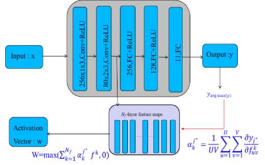
Fig. 1. The Schematic of visualizing LeNet Based Radio Modulation Classifier

• 1.    LeNet Classifier

• 2.    ResNet Classifier

In CNN based radio modulation classifier we use the LeNet based classifier and the ResNet based classifier. The LeNet based classifier consists of two convolutional layers and three fully connected layers. We use the ReLU activation function and the softmax function in the last fully connected layer which predicts the modulation categories. Now we use the feature maps obtained from the last convolutional layer to find the activation vector.

The ResNet based classifier gives greater accuracy than the LeNet based modulation classifier. The ResNet model consists of three residual stack layers and three fully connected layers. The residual stack consists of five convolutional layers and one max pooling layer. Here also the activation vector is computed from the last convolutional layer.

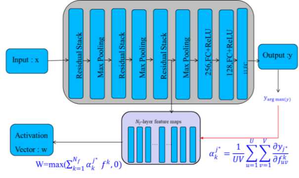
Fig. 2. The Schematic of visualizing LeNet Based Radio Modulation Classifier

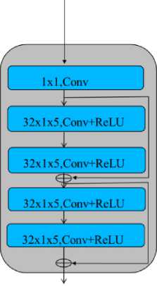
Fig. 3. Residual Stack Structure

• B.    Visualizing LSTM classifier

4.    Real Time Signal Processing

The LSTM is a recurrent neural network which is used in speech recognition, text recognition. The LSTM consists of three gates namely the input gate, forget gate and output gate which is used for prediction. The model consists of two LSTM layers and two fully connected layers by masking the radio samples x and reducing the anticipated probability, an activation vector w. In LSTM we cannot take features from last layer to visualize as of in CNN based classifier. Hence we use a mask function [13-15] and then give those values as input to the LSTM model and find predicted categories from which we can obtain the activation vector w.

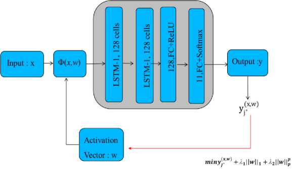
Fig. 4. The Schematic of visualizing LSTM Based Radio Modulation Classifier

For real time signal Processing we used a device name called SDR Receiver. That is most popular one. SDR stands for Software - defined Radio, which is an RF communication system that uses software or firmware to perform signal processing operations that would ordinarily be handled by hardware.

Mixers, filters, amplifiers, modulators, demodulators, and the devices are included in this SDR category. In recent years, Software Defined Radio (SDR) technology has improved dramatically. Hardware advancements have resulted in lower prices and improved performance, which can offer some substantial advantages over traditional hardware-based radio solutions. Software defined radios are being employed in a variety of applications in a variety of fields, especially with the help of signal processing. It also implies that a single hardware platform may be utilised across a wide range of goods and applications, saving money while maintaining or enhancing performance. From SDR receiver we will record a radio signal by using SDR receiver and antenna and then it will give a wav file.

Then we have to interpret the wav file to find out the in-phase (I) and quadrature-phase (Q) values. Now by using the in-phase (I) and quadrature-phase (Q) values we will able to perform the classification and visualization. It is intended for radios experiment and features a wider frequency range of 1 MHz to 6 GHz, as well as a high bandwidth of up to 20 MHz as well as an 8-bit ADC.

The SDR software radio idea may be applied to a variety of situations: these are

• 1.    Military: Software defined radio technology has been successfully adopted by the military, allowing them to reutilize hardware and alter signal waveforms as required.

• 2.    Amateur radio: Radio amateurs have had great success with software defined radio technology, which has enhanced performance and reliability.

• 3.    Research & Development: software defined radio, has shown to be highly valuable in many research endeavours.

Without having to start from scratch, the radios may be modified to give the specific receiver and transmitter needs for every application.

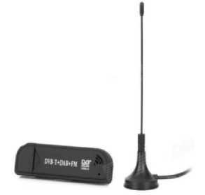
Fig. 5. SDR Dongle Receiver

By using this device we can capture the radio signal around the environment with help of the software named is airspy. By using airspy software we can record the radio signals into a wav file format. Now we have to process the wav file in order to retrieve the data points of the radio signal which can be used for training and testing of radio modulation classifiers.

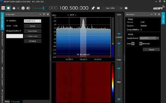
Fig. 6. Airspy SDR sharp studio

Airspy is a popular series of Software-Defined Radio (SDR) receivers that use collaboration of DSP and RF methods to achieve high performance at a reasonable rate. The objective is to satisfy the most discerning telecommunications experts and radio lovers while also providing a viable option to both budget-conscious and high-end receivers. Because of its close integration we use standard free SDR software for signal gathering, analysis, and demodulation, Airspy radios offer global reception accuracy and ease of use.

The above figure shows that airspy platform used for recording radio signals. Here we captured the radio signals of frequency of 100.5MHz which is a local radio station with good signal strength in our environment. Hence we can use this software and hardware to capture the real time radio signals for analysis and further applications.

5.    Result

From the RadioML2016.10b we used six lakhs radio samples of 10 different radio modulation categories with varying signal to noise ratio from 0 to 18 decibel with the step size of two. From this we split the radio samples into training and testing dataset to implement radio modulation classifiers in python platform. The table 1 shows that parameter used in the radio modulation classifiers. We implement LeNet, ResNet and LSTM model have the accuracy of 80%, 70% and 92%.

Table 1. Comparison of the radio modulation classifiers

	Batch Size	Epoch	Optimizer	Accuracy
LeNet	128	150	Adam	80%
ResNet	128	150	Adam	70%
LSTM	128	150	Adam	92%

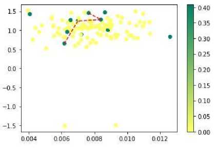
Fig. 7. Visualized LeNet output

-0.35

-030

-0.25

-020

-015

-010

-005

Fig. 8. Visualized ResNet output

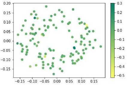
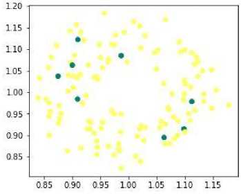
Fig. 9. Visualized LSTM output

The above given figures show the visualized output for the different deep learning based radio modulation classifiers. The fig.7 is the visualized output from the LeNet based radio modulation classifier. The fig.8 is the visualized output from the ResNet based radio modulation classifier. The fig.9 is the visualized output from the LSTM based radio modulation classifier.

6.    Conclusion and Furture Work

In this paper, we offer a visualisation approach for examining the radio features recovered by CNN-based and LSTM-based deep learning-based radio modulation classifiers, respectively. We demonstrate that CNN-based classifiers are unaffected by input signal and capture equivalent radio properties by investigating radio signals in both I/Q and amplitude/phase forms. The transitions between modulation categories are captured by Both the ResNet-based classifier and the LeNet-based classifier are radio modulation classifiers and The classifier is based on the LSTM , on the other hand, discriminates between modulation which is identical to human expert knowledge. Even with short radio samples, to categorise and illustrate multiple deep learning-based modulation classifiers. From the implemented deep learning radio modulation classifiers we obtain higher accuracy of 92% for the LSTM based radio modulation classifier. Hence the LSTM radio modulation classifier is the best among the implemented radio modulation classifiers. In the future we would classify the radio signals with a shorter radio sample and to achieve higher accuracy. This will be easy if we reduce the size of the input to classify the radio signals, it reduces the training and the testing data size.