Deep Learning in Character Recognition Considering Pattern Invariance Constraints

Pattern recognition has been successfully applied in different fields, and the benefits therein are somewhat obvious; in particular, character recognition has sufficed in applications such as reading bank checks, postal codes, document analysis and retrieval etc.

In view of this, several recognition systems exist today, which employs different approaches and algorithms for achieving such tasks. Some common recognition systems approach that have been in use include template matching, syntactic analysis, statistical analysis, and artificial neural networks. The above mentioned approaches to the problem of pattern recognition, and therefore character can be classified into non-intelligent and intelligent systems. If intelligence is “the ability to adapt to the environment and to learn from experience” [1]; then we can say that approaches to pattern recognition such as template matching, syntactic analysis, and statistical analysis are non-intelligent, as they inevitably lack the ability to learn and hence adapt to the tasks they are designed for. Neural networks, conversely, can learn the features of task on which they are designed and trained; they can also adapt to some moderate variations such as noise on the data they have been trained with, hence considered intelligent.

The success of neural networks in contrast to other non-intelligent recognition approaches is striking, based on performance, and somewhat ease of design considering the capability of neural networks in approximation any mapping function of inputs to outputs while requiring ‘least’ domain specific knowledge for its programming each time it is embedded in different applications. i.e. self-programming. The above notion leads to the fact that a new programming algorithm and therefore codes need not necessarily be developed for tasks of at least similar applications as it is done in convectional-digital computing (i.e. same suitable learning algorithms can be used for different tasks); this allows for two options hence:

• •    designers focus more on developing extraction methods for useful features that can be learnt by the network for different tasks which reduces the computational requirement and somewhat increases performance as most irrelevant features to learning would have been filtered out, hence learning is more concise.

• •    more knowledge, features extracting machine learning algorithms and architecture of neural networks that allows the network itself to learn and extract important features from the training data, hence lesser effort from designers in handcrafting features from the training data. This second option has recently boosted interest in machine learning, as marked achievements include emergent various architectures of neural networks that can learn from almost unprocessed data.

Also, the level of intelligence required of recognition systems has gradually changed over the years from basically almost 100% handcrafted and extracted features from data for learning to almost raw data. Some consideration on the amount of common pattern invariance achievable in learning has also changed; such common invariances include relatively moderate translation, rotation, scale mismatch, and noisy patterns. These problems are briefly discussed below.

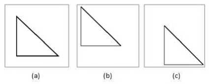
Fig. 1. Translational invariance

It can be seen in the figure above, the linear translations (fig.1 b & c) of the original pattern (fig.1a) in the image; it is obvious that this scenario shouldn’t represent different patterns in an intelligent recognition system, a situation referred to as translational invariance. Although there exist registration algorithms that attempt to align a pattern image over a reference image so that pixels present in both images are in the same location. This process is useful in the alignment of an acquired image over a template [2].

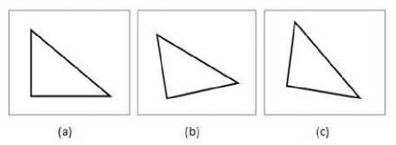
Fig. 2. Rotational invariance

Rotational invariance is shown in fig.2, with (b) and (c) being the rotated versions of (a).

(a)                         (b)                         (c)

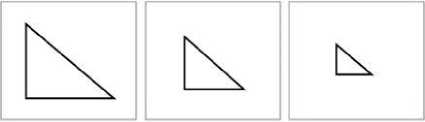
Fig. 3. Scale invariance

Scale invariance is a situation where the size of the pattern has been scaled down or blown up; it is important to note that the actual dimension or pixels of the image remains the same in this situation. e.g. see fig.3.

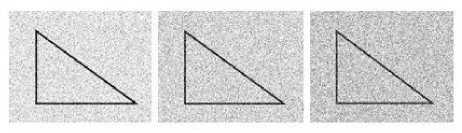
Fig. 4. Noise corruption

Noise, is another problem faced in pattern recognition as shown above; the question of how much is the level of noise required to so corrupt the input as to lead to misclassification of patterns.

It is the aim to design machine learning algorithms and novel neural network architectures that are more robust to pattern invariance and noise etc.

• II.    Related Works

Gorge and Hawkins [3], in their work, ‘Invariant Pattern Recognition using Bayesian Inference on Hierarchical Sequences’, suggested that invariance could be learned in a neural network using Bayesian inference approach. Their work exploited the hierarchical learning and recalling of input sequences at each layer, it was proposed that some lower transformation features learned from some particular patterns could be used for other patterns representation at higher levels; hence making learning more efficient. They employed feedforward and feedback connections, which were described to hold the inferences made on the current (or locally stored) observations and supply computed predictions to the lower levels respectively.

Rahtu E. et al [4] proposed an affine invariant pattern recognition system using multiscale autoconvolution, in which they employed probabilistic interpretation of image functions. It was reported in their work that the proposed approach is more suited for scenarios where distortions present in images can be approximated using affine transformations. Furthermore, their simulation results presented on the classification of binary English alphabets A, B, C, D, E, F, G, H, and I, with added binary noise can be seen to be relatively poor. It was established that the affine invariant moment and multiscale autoconvolution classification approaches presented seem to collapse at a noise level of 2% and 6% respectively, giving high classification errors. Also, it can be seen that such an approach seems to depend on very complex and rigorous mathematical build up, rather than a simple approach of describing invariance learning.

Kamruzzaman and Aziz [5], in their research, presented a neural network based character recognition system using double backpropagation. The classification was achieved in two phases, which involves extracting invariant features to rotation, translation, and scale in the preprocessing phase (first phase); and training a neural network classifier with the extracted features in the second phase. It was recorded that a recognition rate of 97% was achieved on the test patterns .

It was suggested in their work that their classification system was not tested on real world data such as handwritten digits, hence the presented approach could not be verified for robustness in practical applications where many pattern irregularities may make such systems suffer poor performance.

It will be observed that one thing that is common to the above reviewed researches is that they seem to rely more on somewhat complex data manipulations and preprocessing techniques and lesser on an intelligent system that ‘strive’ to simulate how pattern invariance is achieved as obtains in the human visual perception system.

Conversely, this paper takes an alternative approach, by presenting a work which focuses on invariance learning based on the neural network architectures, rather than complex training data manipulation schemes and painstaking mathematical foundations. It is noteworthy that this research did not employ any invariant feature extraction technique; hence, investigates how neural network structures and learning paradigms affect invariance learning. Also, to reinforce the application importance of this work, real life data, ‘handwritten characters’, have been used to train and simulate the considered networks.

Furthermore, one ‘con’ approach to achieving invariance in recognition systems is for any specific object, invariance can be trivially “learned” by memorizing a sufficient number of example images of the transformed object [6].

Unfortunately, the difficulty is to synthesize, and then to efficiently compute, the classification function that maps objects to categories, given that objects in a category can have widely varying input representations [7]; bearing in mind also that this approach increases computational load on the designed system.

A better approach is to consider neural network architectures that allow some level of built-in invariance due to structure; and of course, this can usually still be augmented with some handcrafted invariance achieved through data manipulation schemes.

Recent experimental findings demonstrating that distributed neural populations (e.g. deep networks) in early visual processing areas are recruited in a targeted fashion to support the transient maintenance of relevant visual features, consistent with the hypothesis that shortterm maintenance of perceptual content relies on the persistent activation of the same neural ensembles that support the perception of that content [8], [9], [10].

Neural networks of different architectures have been used in various machine learning assignments of pattern recognition; usually, involving just a single hidden layer. Although, it was later hypothesized the benefits of having networks with more than a single hidden layer, and there have been past research attempts to adopt multilayer neural networks, but technical difficulties encountered in training such networks led to the lost of interest by researchers for a while as presented in the following section.

It is the hope that simple, novel and emerging neural network architecture and learning algorithms can overcome or cope with some major pattern invariances as have been discussed. So far, one of the most successful pattern recognition systems in machine learning is deep neural networks, and is discussed briefly in section III.

• III.    Deep learning

• A.    Insight into deep learning

Deep learning depicts neural network architectures of more than a single hidden layer (multilayer networks); in contrast to networks of single hidden layer which are commonly referred to as shallow networks. These networks enjoy some biologically inspired structure that overcomes some of the constraints and performance of shallow networks. Such features include:

• •    distributed representation of knowledge at each hidden layer.

• •    distinct features are extracted by units or neurons in each hidden layer.

• •    several units can be active concurrently.

Generally, it is conceived that in deep networks, the first hidden layer extracts some primary features about the input, then these features are combined in the second layer to more defined features, and these features are further combined into well more defined features in the following layers, and so on. This can be somewhat seen as a hierarchical representation of knowledge; and obvious benefits of such networks compared to shallow networks include capability to search a far more complex space of functions as we stack more hidden layers in such networks.

Of course, such an elaborate and robust structure didn’t come without a price of difficultly in training.

At training time, small inaccuracies in other layers may be exploited to improve overall performance, but when run on unseen test data these inaccuracies can compound and create very different predictions and often poor test set performance [11].

Common problems associated with training deep networks conventionally (through backpropagation algorithm) are discussed below.

• •    Saturating units: this occurs when the value of the preactivations of hidden units are close to 1, such that the error gradient propagated to the layer below is almost 0.

• •    Vanishing gradients: since deep networks are basically multilayer networks, and trained with gradient descent by back propagation of errors at the output; it therefore follows that there is a ‘dilution’ of error gradients from a layer to the one below as a result of saturating units in the present layer; this consequently slows down or hamper learning in the network. Research works have shown that Hyperbolic-Tangent, Softsign [12], and Rectified Liner activations have improved performance on units saturation [13].

• •    Over-fitting: Since as we stack more hidden layers in the network, we add more units and interconnections, therefore, the feasibility of the network memorizing input patterns grows. Hence, in as much as we achieve distributed knowledge with more hidden layers, it comes with a trade-off of over-fitting. This problem is usually solved using various learning validation schemes during training (i.e. monitoring the error on the validation data) and different regularization algorithms; one method that has sufficed in this situation is the drop-out technique (removing units and their corresponding connections temporarily from the network) that prevents overfitting and provides a way of approximately combining exponentially many different neural network architectures efficiently [14].

Drop-out technique is a more recent approach where hidden units are randomly removed with a probability of 0.5 as this has been seen to prevent the co-adaptation of hidden units [15].

Erhan also noted in his work that pre-training is a kind of regularization mechanism [16].

Under-fitting: Since stacked architectures have usually thousands of parameters to be optimized during training, the feasibility of the network converging to a good local minimum is hence consequently reduced.

Back-propagation networks are based on local gradient descent, and usually start out at some random initial points in weight space. It often gets trapped in poor local optima, and the severity increases significantly as the depth of the networks increases [17]. Several optimization algorithms have been proposed to this problem such as different pre-training schemes for initializing the networks’ memory.

• B.    Classification of deep learning architectures

• •    Generative Architectures

This class of deep networks is not required to be deterministic of the class patterns that the inputs belong, but is used to sample joint statistical distribution of data; moreover this class of networks relies on unsupervised learning. Some deep networks that implement this type architecture include Auto Encoders(AEs), Stacked Denoising Auto Encoders(SDAE), Deep Belief Networks (DBNs), Deep Boltzmann Machines (DBMs) etc.

In general, they have been quite useful in various non-deterministic pre-training methods applied in deep learning and data compression systems.

• •    Discriminative Architectures

Discriminative deep networks actually are required to be deterministic of the correlation of input data to the classes of patterns therein. Moreover, this category of networks relies on supervised learning. Examples of network that belong to this class include Conditional Random Fields (CRFs), Deep Convolutional Networks, Deep Convex Networks etc. In as much as these networks can be implemented as ‘stand-alone’ modules in applications, they are also commonly used in the finetuning of generatively trained networks under deep learning.

• •    Hybrid Architectures

Networks that belong to this class rely on the combination of generative and discriminative approach in their architectures. Generally, such networks are generatively pre-trained and then discriminately finetuned for deterministic purposes. e.g. pattern classification problems. This class of networks has sufficed in many applications with the state-of-art performances.

• IV.    Trainiing Deep Learning Models

• A.    Stacked denoising auto encoder (SDAE)

Stacked Auto Encoders (SDAEs) are basically multilayer feedforward networks with the little difference being the manner in which weights are initialized. Here, the weights initialization is achieved through a generative learning algorithm, as this provides good starting weight parameters for the network (and helps fight under-fitting during learning).

An auto encoder (single layer network) is a feedforward network trained to replicate the corresponding inputs at the output. During training, these networks learn some underlying features in the training data that are necessary for the reproduction at the output layer. The target outputs of these networks are the corresponding inputs themselves. i.e. no labels, hence an unsupervised learning.

The application of auto encoders and therefore generative architectures leverage on the unavailability of labelled data or the required logistics and cost that may be necessary in labeling available data. It therefore follows that generative learning suffices in situations where we have large unlabelled data and small labelled data. The unlabelled data can be used to generatively train the network as in the case of auto encoders and the small labelled data used in the fine-tuning of the final network (as in hybrid networks).

lnPut                                         Output

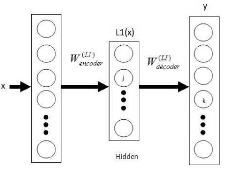
Fig.5. Auto encoder

As can be seen above (fig.5), the auto encoder can be decomposed into two parts, the encoder, and decoder. It will also be noted that the number of output and input neurons, k, are equal (since the input and output are the same, hence of the same dimension), while the number of hidden units, j, is smaller than k, generally. i.e. a sort of data compression scheme can be inferred.

The auto encoder can be seen as an encoder-decoder system, where the encoder (input-hidden layer pair) receives the input, extracting essential features for reconstruction; while the decoder (hidden-output layer pair) part receives the features extracted from the hidden layer, performing reconstruction at its best.

Auto encoders can be stacked on one another to achieve a more distributed and hierarchical representation of knowledge extraction from data; such architectures are referred to Stacked Auto Encoders (SAEs).

Some undeveloped features are extracted in the first hidden layer, followed by more significant elementary features in the second, to more developed and meaningful features in the subsequent layers.

The training approach that is used in achieving learning in generative network architectures is known as ‘greedy layer-wise pre-training’. The idea behind such an approach is that each hidden layer can be hand-picked for training as in the case of single hidden-layer networks; after which the whole network can be coupled back as whole, and fine-tuning done if required.

Since the auto encoder is fundamentally a feedforward network, the training is described below.

Encoder mode:

L1( x ) = g ( m ( x »= sigm ( ь ( L 1) + WeLc) _der x )

^y = z ( n ⁽ x )) = sigm ^{( ь (} y ) + WdLOderL¹ x ))

Where, m(x) and n(x) are the pre-activations of the hidden and output layers L1 and y respectively; b(L1) and b(y) are biases of the hidden and output layers L1 and y respectively.

The objective of the auto encoder is to perform reconstruction as “cleanly” as possible, which is achieved by minimizing cost functions such as are given below.

k

C(x, y) = ^(Ук - xk )2

¹                                              (3)

k

C ⁽ x , У) = - E ⁽ x k log( У к ) + ⁽¹ - x k ) ^log(1 - У к ))    ⁽⁴⁾

Equation 3 is used when the range of values for the input are real, and a linear activation applied at the output; while equation 4 is used when the inputs are binary or fall into the range 0 to 1, and sigmoid functions are applied as activation functions. Equation 4 is known as the sum of Bernoulli cross-entropies.

In the greedy layer-wise training, the input is fed into the network with L1 as the hidden layer and L2(x) as the output; note that L2(x) has target data as the input. The network is trained as in back propagation and weights connection between the input layer and L1 saved or fixed (fig.6).

The input layer is removed and L1 made the input, L2 the hidden layer, and output follows last (i.e. layer y). The activation values of L1 now act as input to the hidden layer L2(x), and the output layer made the same as input L1(x), weights between L1(x) and L2(x) are trained and fixed.

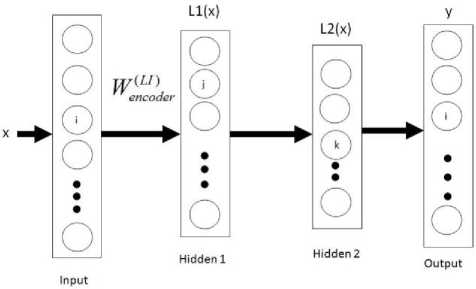
Fig. 6. Stacked auto encoder

Finally, the pre-trained weights obtained from the greedy layer-wise training are coupled back to the corresponding units in the network so that final weights fine-tuning for the whole network can now be carried out using back propagation algorithm. i.e. the original training data is supplied at the input layer and the corresponding target outputs or class labels are supplied at the output layer. Note that the weights between the last hidden layer and the output network can either be randomly initialized or trained discriminatively before the final network fine-tuning.

Another variant of auto encoders, known as denoising auto encoders is very similar to the typical auto encoder except that the input data are intentionally corrupted by some moderate degree (setting some random input data attributes to 0) and while the corresponding targets are the correct, unaltered data. Here, the denoising auto encoder is required to learn the reconstruction of corrupt input data; this greatly improves the performance of initialized weights for deep networks.

Denoising is advocated and investigated as a training criterion for learning to extract useful features that will constitute better higher level representation [18].

• B.    Deep belief network (DBN)

A DBN is a deep network, which is graphical and probabilistic in nature; it is essentially a generative model too.

A belief net is a directed acyclic graph composed of stochastic variables [19].

These networks have many hidden layers which are directed, except the top two layers which are undirected.

The lower hidden layers which are directed are referred to as a Sigmoid Belief Network (SBN), while the top two hidden layers which are undirected are referred to as a Restricted Boltzmann Machine (RBM). i.e. fig.7. Hence a DBN can be visualized as a combination of a Sigmoid Belief Network and a Restricted Boltzmann Machine. The sigmoid belief network is sometimes inferred as a Bayesian network or casual network [20].

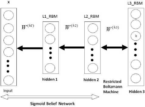
Fig. 7. Deep Belief Network

Furthermore, it has been shown that for the ease of training, deep belief networks can be visualized as a stack of Restricted Boltzmann Machines [21] [22].

Since the last two layers of a deep belief network is an RBM, which is undirected, it can therefore be conceived that a deep belief network of only two layers is just an RBM. When more hidden layers are added to the network, the initially trained deep belief network with only 2 layers (also just an RBM) can be stacked with another RBM on top of it; and this process can be repeated with each new added layer trained greedily.

Such a training scheme is aimed at maximizing the likelihood of the input vector at a layer below given a configuration of a hidden layer that is directly on top of it.

As discussed above, it is therefore essential to introduce Restricted Boltzmann Machine for the proper understanding of deep belief networks.

A restricted Boltzmann machine has only two layers (fig.8); the input (visible) and the hidden layer. The connections between the two layers are undirected, and there are no interconnections between units of the same layer as in the general Boltzmann machine. We can therefore say that from the restriction in interconnections of units in layers, units are conditionally independent.

The RBM can be seen as a Markov network, where the visible layer consists of either Bernoulli (binary) or Gaussian (real values usually between from 0 to 1) stochastic units, and the hidden layer of stochastic Bernoulli units [22].

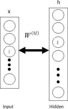
Fig.8. Restricted Boltzmann Machine

The main aim of an RBM is to compute the joint distribution of v and h, p(v,h), given some model specific parameter, ϕ.

This joint distribution can be described using an energy based probabilistic function as shown below.

E(x,h;φ)=-∑∑Wijxihj -∑bixi - ∑bjhj (5)

ij           ij

_e ( - E ( x , h ; φ ))

p(x, h;φ) =

Z = ∑i∑he(-E(x,h;φ))

Where, E(x,h;ϕ) is the energy associated with the distribution of x given h, x and h are input and hidden units activations respectively, i is the number of units at the input layer, j is the number of units at the hidden layer, bi is the corresponding bias to the input layer units, bj is the corresponding bias to the hidden layer units, Wij is the weight connection between unit xi and hj, P(x,h;ϕ) is the joint distribution of variable x and h, while Z is a partition constant or normalization factor [22] [23].

For a RBM with binary stochastic variables at both visible and hidden layers, the conditional probabilities of a unit, given the vector of unit variables of the other layer can be written as,

p(hj =1| v;φ) = σ(∑Wijxi +bj) (8)

i

p(xi =1| h;φ) = σ(∑Wijhj +bi) (9)

Where σ is the sigmoid activation function.

Deng observed in his work that by taking the gradient of the log-likelihood p (x,h; ϕ), the weight update rule for RBM becomes,

^W =Еа ДхкЛ-Е дЛх1гЛ (10)

ij data i j mod el i j

Where, E data is the actual expectation when h j is sampled from x, given the training set; and E model is the expectation of h j sampled from x i , considering the distribution defined by the model.

It has also been shown that the computation of such likelihood maximization, E model , is intractable in the training of RBMs, hence the use of an approximation scheme known as “contrastive divergence”, an algorithm proposed to solve the problem of intractability of E model by Hinton [21].

Because of the way it is learned, the graphical model has the convenient property that the top-down generative weights can be used in the opposite direction for performing inference in a single bottom-up pass [24].

Hence, such an attribute as mentioned above makes feasible the use of an algorithm like backpropagation in the fine-tuning or optimization of the pre-trained network for discriminative purpose.

• V.    Data Analysis For Learning

As the aim of this research is to investigate the tolerance in neural network based recognition systems to some common pattern variances that occur in pattern recognition; the variances that have been considered include rotation, translation, scale mismatch, and noise. Handwritten Yoruba vowel characters have been used to evaluate and observe the performance of the different network architectures considered for this work.

Yoruba language is one of the three major languages in Nigeria with over 18 million native users; used largely by the southwestern part of the country. It consists of 7 vowel alphabet characters, and in recent years, the acceptance and usage of the language have grown to such an extent that Google now accepts web searches using the language. It is noteworthy that the patterns (Yoruba vowel characters) that have been used in this work are quite harder for recognition than some other languages, as some of the characters comprise diacritical marks; these marks can lie in slightly different positions of interest and also that the writing styles of individuals makes recognition even tougher.

Handwritten copies of the characters are collected and processed into a form that is suitable to be fed as inputs to the different trained networks; different databases with specific variances were also collected to evaluate the performance of the trained networks on such variances. Listed below are the different collected databases and logic of sequence applied to this research.

• •    Training database of Yoruba vowel characters: A1

• •    Validating database of Yoruba vowel characters: A2

• •    Translated database of Yoruba vowel characters: A3

• •    Rotated database of Yoruba vowel characters: A4

• •    Scale different database of Yoruba vowel character :

A5

• •    Noise affected database of Yoruba vowel character: A6

• •    Process image databases as necessary

• •    Train and validate all the different networks with created databases A1 and A2 respectively.

• •    Simulate the different trained networks with A3, A4, A5, and A6.

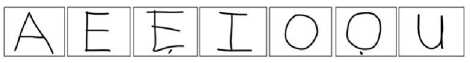
Fig. 9. Unprocessed character images

All original databases contain images with 300×400 pixels; the figure above shows separate handwritten character images which have not been processed.

The characters were processed by binarizing the images (black & white), obtaining the negatives, and filtering using a 10×10 median filter; finally all images were resized to 32×32 pixels to be fed as inputs to the different designed networks. All networks have 7 outputs neurons as can be deduced from the number of characters to be classified.

• A.    Databases A1 and A2

These databases A1 and A2 contain the training and validation samples, respectively, for the different network architectures considered for this research. The characters in these databases A1 and A2 have been sufficiently processed with the key interest being that images are now centered in the images i.e. most redundant background pixels removed.

вяжюнаяиж ЗИЙИЖМКЖВ® ИИЯбИймВЙН жюийжкаяе

Fig.10. Training and validation characters

• B.    Database A3

For the purpose of evaluating the tolerance of the trained networks to translation a separate database was collected with the same characters and other feature characteristics in databases A1 and A2 save that the characters in the images have now been translated horizontally and vertically. The figure below describes these translations.

А ЕЕ 100 U

Fig. 11. Translated characters.

• C.    Database A4

This database contains the rotated characters contained in database A1 and A2. Its sole purpose is to further evaluate the performance of trained networks on pattern rotation. See fig.12 for samples.

Fig. 12. Rotated characters

• D.    Database A5

This database is essentially databases A1 and A2 except that the scales of characters in the images have now been purposely made different in order to evaluate the performance of the networks on scale mismatch. It will be seen that some characters are now bigger or smaller as compared to the training and validation characters earlier shown in Fig.10.

Fig.13 show samples contained in this database.

Fig.13. Scale varied characters

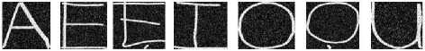
• E.    Database A6

Database A6_1:

Database A6_2:

Database A6_3:

Database A6_4:

Database A6_5:

• 2.5% noise density 5% noise density 10% noise density 20% noise density 30% noise density

The figure below show character samples of database A6 4.

• VI.    Deep Networks Test and Analysis

The tables below show the error rates obtained by simulating the trained networks with the different databases as described in the section V.

It is to be noted that the trained networks were only trained with the database A1 and validated with database A2 to prevent overfitting.

All the databases images were resize to 32×32 pixels and then reshaped to a column matrix of size 1024×1 which were found suitable to be fed as network inputs. All the networks have 7 output neurons to accommodate the number of classes of the characters.

The networks that were trained include the conventional Back Propagation Neural Network (BPNN), Denoising Auto Encoder (DAE), Stacked Denoising Auto Encoder (SDAE), and Deep Belief Network (DBN).

The BPNN networks were trained on the scaled conjugate algorithm; using 1 (BPPN-1) and 2 (BPNN-2) hidden layers to observe the effect of deep learning on pattern invariances of interest as discussed in the previous sections.

The DAE and SDAE networks were trained with a 0.5 input zero mask fraction. i.e. denoising parameter.

14,000 samples have been used to train the networks, 2,500 samples as the validation set, and 700 samples as test set for each invariance constraint.

Please note that as some of the original images were rotated to create a larger database for training, validation, and testing; thus inferring that some level of prior knowledge on rotation of characters have been built into the network; nevertheless the performance of the trained networks was still verified on rotational invariance.

Also important, is that the only variance introduced into each database A3, A4, A5, and A6 is the particular invariance of interest correspondingly, as this allows the sole observation of network tolerances on a particular invariance. Below are the network training parameters and achieved error rates.

Table 1. Training parameters for networks

No. of hidden neurons	1st layer	2nd layer
BPNN – 1 layer	65	0
BPNN – 2 layers	95	65
DAE – 1 layer	100	0
SDAE – 2 layers	95	65
DBN - 2 layers	200	150

Table 2. Error rates for training and validation data

Nets.	Train	Validate
BPNN – 1 layer	0.0433	0.0734
BPNN – 2 layers	0.0277	0.0639
DAE – 1 layer	0.0047	0.0679
SDAE – 2 layers	0.0028	0.0567
DBN - 2 layers	0.0023	0.0377

It can be seen from table 2 that the DBN achieved the lowest error rate on both the train and validation data. The SDAE comes second in performance to the DBN on classification error rates. While the AE outperformed the BPNN-1 on both train and validation error rates, it can be inferred that the pre-training schemed allowed the weights initialization of the AE to occur in a weight space which was more favourable to the convergence of the network to a better local optimum, as compared to BPNN-1 without pre-training.

Table 3. Error rates for network architectures on variances

Nets.	Translation	Rotation	Scale
BPNN – 1 layer	0.8571	0.3140	0.3571
BPNN – 2 layers	0.8286	0.2729	0.3658
DAE – 1 layer	0.8000	0.2486	0.3057
SDAE – 2 layers	0.7429	0.2214	0.2743
DBN - 2 layers	0.8143	0.1986	0.2329

The simulation results on the considered invariances for the different trained networks are shown in table 3. It can be seen that the SDAE has the lowest error rate on translation, while the DBN outperformed other networks on rotational and scale invariances.

It can be observed that the two best networks in invariance learning (DBN and SDAE) are of 2 hidden layers, hence we can conjure that these networks were able to explore a more complex space of solutions while learning to the deep nature; since hierarchical learning allows more distributed knowledge representation.

Table 4. Error rates for network architectures on noise

Nets.	2.5%	5%	10%
BPNN – 1 layer	0.3214	0.3486	0.3471
BPNN – 2 layers	0.2943	0.3158	0.3414
DAE – 1 layer	0.2843	0.3243	0.4357
SDAE – 2 layers	0.2586	0.3043	0.3857
DBN - 2 layers	0.2371	0.2771	0.3843

Table 5. Error rates for network architectures on noise

Nets.	20%	30%
BPNN – 1 layer	0.4129	0.4829
BPNN – 2 layers	0.4486	0.5586
DAE – 1 layer	0.5986	0.6843
SDAE – 2 layers	0.5386	0.6371
DBN - 2 layers	0.6414	0.7729

The figure below shows the performance of the different network architectures at 0%, 2.5%, 5%, 10%, 20%, and 30% noise densities added to the test data.

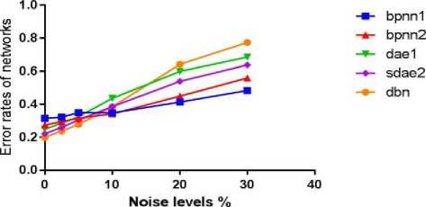
Fig. 15. Performance of networks on noise levels

DBN and SDAE have low error rates at relatively low noise levels, but their performances seem to degrade drastically from 7% and 10% noise densities respectively (see fig.15). BPNN-1 was observed to have the best performance at 30% noise level.

• VII.    Conclusion

This research is meant to explore and investigate some common problems that occur in recognition systems that are neural network based. It will be seen that the deep belief networks on the average, performed best compared to the other networks on variances like translation, rotation and scale mismatch; while its tolerance to noise decreased noticeably as the level of noise was increased as shown in table 4, table 5, and fig.15.

A noteworthy attribute of the patterns (Yoruba vowel characters) used in validating this research is that they contain diacritical marks which increases the achievable variations of each pattern, and as such, recognition systems designed and described in this work have been tasked with a harder classification problem.

The performances of the denoising auto encoder (DAE-1 hidden layer) and stacked denoising auto encoder (SDAE-2 hidden layer), on the average with respect to the variances in character images seems to second the deep belief network.

The performance of the denoising auto encoder is lower than that of the stacked denoising auto encoder, it can be conjured that the stacked denoising auto encoder is less sensitive to the randomness of the input; of course the training and validation errors for the SDAE are also lower to the DAE, and the tolerance to variances introduced into the input significantly higher. i.e. a kind of higher hierarchical knowledge of the training data achieved.

It is the hope that machine learning algorithms and neural network architectures, which when trained once, perform better on invariances that can occur in the patterns that they have been trained with can be explored for more robust applications. This also obviously saves time and expenses in contrast to training many different networks for such situations.

Furthermore, building invariances by the inclusion of all possible pattern invariances which can occur when deployed in applications during the training phase is one solution that has been exploited; unfortunately this is not always feasible as the capacity of the network is concerned. i.e. considering number of training samples enough to guarantee that proper learning has been achieved.

It can be seen that the major problem in deep learning is not in obtaining low error rates on the training and validation sets (i.e. optimization) but on the other databases which contain variant constraints of interest (i.e. regularization). These variances are common constraints that occur in real life recognition systems for handwritten characters, and some of the solutions have been constraining the users (writers) to some particular possible domains of writing spaces or earmarked pattern of writing in order for low error rates to be achieved.

It has been shown that another flavour of neural networks, “convolutional networks” and its deep variant give very motivating performance on some of these constraints [25], however the complexity of these networks is somewhat obvious.

This work reviews the place of deep learning, a simpler architecture (with no invariant features extraction preprocessing techniques applied), in a more demanding sense, that is, a “train once-simulate all” approach; and how well these networks accommodate the discussed invariances. It is the hope that with the emergence of deep learning architectures and learning algorithms that can extract features that are less sensitive to these constraints, a new era in deep learning, neural networks and machine learning field could emerge in the near future.