Defending against Malicious Threats in Wireless Sensor Network: A Mathematical Model

Published Online February 2014 in MECS

Wireless sensor networks are the emerging technology of this era. The network is composed of hundreds or thousands of self-powered tiny sensor nodes which gather information or detect special events and communicate via radio transmitter or receivers, with the end goal of handing their partially processed data to the base station [1]. Sensing, processing and communication in one tiny device gives rise to a vast number of applications such as environmental monitoring, target  tracking,  micro-surgery, home applications, virtual keyboards, monitoring disaster area, vehicle tracking etc. We focus on security of sensor network because it is vital to the acceptance of WSN in many applications. Thousands of sensor nodes are deployed without any topology overhead it can be placed one by one either by human or robot, or can be deployed by dropping from a plane. The major concern in WSN is that wireless signal cannot be control physically [2] and gives easy access to the attackers. The virus like CABIR [3] and MABIR [4] has ability to spread over the air interface, which make it possible to develop a worm for sensor network. Sensor network are densely deployed and exchange data via short range radio technology which helps worms to propagate without internet connection [5]. Thus, we require robust security mechanism that can defend sensor network against malicious attacks. The sensor nodes are distributed over the monitored region called sensor field as shown in the fig. 1. These scattered nodes are responsible for sensing and transmitting data to the base station. The base station communicates with the end user via internet or satellite [1].

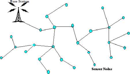
f ig . 1: s ensor nodes sense and exchange data of the monitored region

The journey so far in the development of mathematical worm propagation has been studied using the epidemiological modeling [6-8,9,10] in which the disease status are divided into different compartments which is initiated by Kermack and McKendrick [11] and later extended by Bailey ,Anderson and May [12,13]. The SIS (Susceptible-Infected-Susceptible) and SIR (Susceptible-Infected-Recovered) models are highly applicable and suggested model, SIR model assumes that once a host recovers from the disease, it becomes immune forever while the SIS model has been used for diseases where repeat infections are common. Richard and Mark [14] have proposed an improved SEI

(Susceptible-Exposed-Infected) model to simulate virus propagation in peer to peer network. The SEIR model proposed by Yan and Liu[15] assume that the recovered hosts have a permanent immunization period with a certain probability, which is not consistent with real situation. Kermack and McKendrick classical SIR epidemic model [11] approach was applied to e-mail propagation schemes[10] and modification of SIR models generated guides for infections prevention by using the concept of epidemiological threshold [68][16,17]. To overcome the limitation, Mishra and Saini [6] present a SEIRS model with latent and immune periods, which can reveal common worm propagation. Recently, more research attention has been paid to the combination of virus propagation models antivirus countermeasures to study the prevalence of virus, for example, virus immunization [18] and quarantine[9] have been introduced into such model. The classical models of Kermack and Mc Kendrick [11] have been further applied to specialised networks including sensor networks and ad hoc networks. Computer viruses and worms, and biological viruses show similarity regarding their self-replicating and propagation behaviors. The epidemic models are extensively used by researchers [5, 10] to study the spread of malware in WSN. Some of the related applications of epidemic models in wireless environments have been discussed in the recent literature [20].

The paper is organized as follows: Section 1 deals with Introduction, epidemic model is developed in Section 2, Numerical simulations are performed in section 3, and finally the conclusion is given in section 4.

• II.    Seiqrs-V Epidemic Model

We propose Susceptible -Exposed – Infectious – Quarantine-Recovered-Susceptible with Vaccination compartment (SEIQRS-V) to describe the dynamics of worm propagation with respect to time in WSN. We assume inclusion of new sensor nodes and crashing of the nodes due to the infection of worms or hardware/software failure. Initially we assume all the nodes in the sensor field to be susceptible towards worm infection. Before the sensor nodes become fully infectious its normal performance is affected like slow processing speed etc. such nodes are put into exposed compartment. The nodes having infectious behavior are address by dynamic quarantine where the most infected nodes are isolated from the network till they get recovered. Vaccinating the nodes in a group immunized them toward the worm infection and enabling guideline for typical active worm control.

Let S(t), E(t), I(t), Q(t), R(t) and V(t) denote the number of Susceptible, Exposed, Infectious, Quarantine, Recovered , Vaccinated nodes at time t respectively.

Assume N(t) = S(t) + E(t) + I(t) + Q(t) + R(t) + V(t) for all t.

Where Λ the inclusion of new sensor node in the population, d is the mortality rate of the sensor nodes due to hardware/software failure, δ is the crashing rate due to attack of malicious objects, β is the infectivity contact rate, γ is the rate of transmission from E-class to I-class, α is the rate of transmission from I-class to Q-class, ϕ is the rate of transmission from I-class to R-class, η is the rate of recovery, ε is the rate of transfer from R-class to S-class, ρ is the rate of transmission from V-class to S-class, σ is the vaccinating rate coefficient for the susceptible nodes.

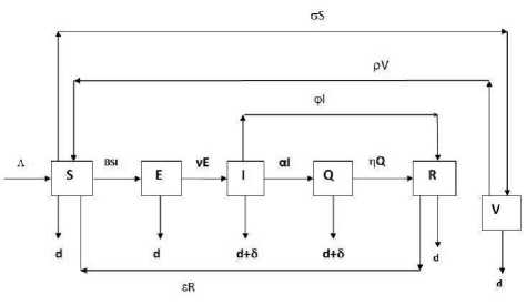
Fig. 2: Schematic diagram for the flow of worm in sensor network

The system of differential equations as per our assumptions, which is depicted in fig. 2, is given as:

• =    Л — 0SI — (а + d)S + eR + pV

• =    P^SI—(Y + ^d)^E

~ = yE — ( (x + p + d + S)I                 (1)

• ^ = aI — (n + d + 6)Q

^ = pI + n Q — ⁽e + d)R

^ = aS — (p + ^V

Now, the total population size is, ™" = Л — (IN — SI

In the absence of attack, the population size of the node approaches the carrying capacity A /d . The differential equation for N implies that solution of (1) starting in the positive orthan R⁺ 6 approaches, enter or remain in the epidemiologically meaningful subset.

D = {(S, E, I, Q , R , V)/(S, E, I , Q , R , V) > 0, S + E + I + Q + R + V <  A /d}

Thus, it suffices to consider solutions in region D. Solution of the initial value problem starting in D and defined by (1) exist and are unique on maximal interval [21]. Since solution remain bounded in the positively invariant region D, the maximal interval is(0, “). Thus,

initial value problem is well posed both mathematically and epidemiologically.	E»-( dX«) ' 0 , °- 0 - 0 - (,+№+d)   ap) If R0 > 1 , then D contains a unique positive,
2.1 Existence and Stability of Equilibrium The system has two possible equilibria in D where, D = {(S,E,I,Q ,R ,7) £R^ :S + E + I + Q+R + V <  N }. The disease free equilibrium for worm free state	endemic equilibrium E * = (S * ,E * , I*, Q *, R *, V * ) Where, *_ e(Y + d) Sy

Е *

(а + ф + d + 5)( n + d + 6)(е + d)

Y{ф(( n + d + 6) + a}YE - 0 (у + d)( n + d + 6)(е + d)

[0 ⁽ у + d)            pa

I —i ^(a+d)- p+d) ^-YA]

I *=

( n + d + <5")( e + d )

Ф( П + d + 6) + a}YE - 0(у + d)( n + d + 6)(e + d)

[ 0 ⁽ y + d)

[—— i(a+d)

"?TdH ^A ]

a (n + d + 5)( e + d)

0 *= -----:--—-:----:--=---:----—---—----:--—---—

( n + d + 6){ф( п + d + 6) + a}yE - 0(у + d)( n + d + 6)(e + d)

0(y + d)           pa e { ■■d'p+:} YA

„* о 9 ⁽ у + d)

* =*

p + d     Уу

Where 6=(a + ф + d + 5)

Thus, we have:   N*=S*+E * +I * + Q * +R * +7 *

• 2.2    The Basic Reproduction Number (R0)

• 2.3    Stability of the Worm Free Equilibrium State

It is defined as the expected number of new cases of infection caused by a typical infected individual. It can be obtained by calculating V and F, where V is the rate of transfer of nodes inside and outside of the infectious compartment and F be the rate of new infection in compartment. Hence, by the equations we obtain,

	-( Y + d)	0	0
V=	Y	-(a + ф + d + 6)	0
	0	a	-( n + d + 6)
	■ 0 У   0
F=	0  0  0
	.0   0    0.

The basic reproduction number is defined as the dominant Eigen value of F V~ ¹ that is,

R .-Si----

( + )( +

To get the stability of the worm free equilibrium state, the Jacobian matrix, of the system (1) that is:

	Г -(a + d)     0         - -S ^ ^ ^^           0           E         pl
	v      7                         d ( p + a +d)                                              M
	0      -(Y + d)        -5 ^ ( 2 +;)-              0            0          0
	d ( p + a +d)
J=	0        Y     -(a + ф + d + 6)       0          0        0	(2)
	0         0            a         -( n + d + 6)     0         0
	0         0            ф               n        -(E + d)     0
	La       0          0            0         0    -(p + d)J

The Eigen values of (2) are:

-(a + d) , -(Y + d) , -(a + ф + d + 6) , -( n + d +

6), -(E + d), -(P + d)

Which all are negative hence the system is locally asymptotically stable at worm free equilibrium point E 0.

Lemma 1: If R 0 1, the worm free equilibrium point E₀ is locally asymptotically stable. If R₀=1, E₀ is stable. If R 0 >1, E 0 is unstable.

Let,

/ „ =lim t_„ inf _e>t / (0), / ” =lim t^„ sup _e >  / (0)

Lemma 2 : Assume that a bounded real valued function ƒ :[0, ∞ ]→R be twice differentiable with bounded second derivative. Let k→∞ and ƒ (t k) converges to ƒ ^∞ to ƒ ∞ then, lim k→∞ ƒ ` (t k) = 0

Theorem 1: if R 0 <1 then worm free equilibrium E 0 is globally asymptotically stable.

Proof: From the system (1) we have,

S(t)5X№ dP+PSd> ^{+ E} , for'> t o

Thus, S" 5 ,::5<

Let c >0 then S " 5 -Л^C^^+d-

(p+и+d)

Similarly the second equation of the system (1) can be expressed as

dS

< Л dt

—

d ⁽ p + о + d) p + d

dE = ^л A Cp+d) ) — (y + d)E             (3)

dt и Vd(p+n+d)

A solution of the equation — < Л — dp+n—)X is a 1        dt           p+d super solution of S(t).

Since X(t)> ^(P++d) as t>", then for given ^E >0, such that

Using this the 3rd and 4th equation of the system(1) we have,

■ Е

■ I

■ Q

5 P [QI

, where

I A ⁽p+d)

^{—(Y + d)}     Pbs+nzs )

Y    —(a + ф + d + 3)0             a

—

00(П + d + 6)

I

let M ∈ R⁺, such that

M > max{(Y + d), (a + ф + d + 6), ( n + d + 6)} .

Thus, ρ+MI 3×3 is a strictly positive matrix where I 3x3 is an identity matrix. If ω 1 , ω2, ω 3 are the Eigen value of ρ, then ω1+M, ω2+M, ω3+M are the Eigen value of ρ+MI 3×3 . Thus, from the Perron-Frobenius theorem[22],

ρ+MI 3 has a simple positive Eigen value equal to dominant Eigen value and corresponding Eigen vector e >0, which implies that, ω 1 , ω 2 and ω 3 are real. If ω 1 + M is the dominant Eigen value of ρ+MI3x3, then ω 1 > ω 2 and ω 1 > λ 3, and e ρ= e ω 1 . Obviously ω 1 , ω 2 and ω 3 are the roots of equation.

to2 + (2d + a + y + Ф + 3 +)w + (y + d)(a +ф + d + 3) — (^Ad+d)]) = 0         (5)

Since R 0< 1 for ∈ >0, sufficiently small, we have,

⁽ Y + d) ⁽ " ⁺ » ^{+d + 3 )} —R^) > ⁰

Therefore coefficients of the quadratic equation (5) are positive.

Thus ω 1 , ω 2 and ω 3 are negative. So from equation (4) for t≥t 0

d

- (e. [E(t),I(t),Q(t)]) < to1.e[E(t),I(t),Q(t)]

Integrating the above inequality, we get,

05 e. [E(t),I(t),Q(t)]< e. [E(t J,I(t J, Q(t!) ]e“ 1(Etd) , for t > t1 > t0.

Since ω1<0,  .[E(t 1 ),I(t 1 ),Q(t 1 )]→0 as t→∞

Using e>0, we have,

[E(t), I(t), Q(t)]>(0,0,0) as t>"

By Lemma 2 , we choose a sequence t n →∞ , S n →∞(n→∞), such that

S(S n )→S^∞, S(t n )→S ∞ , S(S n )→0, S(t n )→0

Since E(t),I(t)→Q(t)→0 as t→∞, thus from the first equation of system (1) ,We have, limn>"S(t)=

A (p+d) d (p+ a +d)

Hence by incorporating lemma 1, the worm free equilibrium E₀ is globally asymptotically stable, if R₀<1.

• III.    Numerical Results

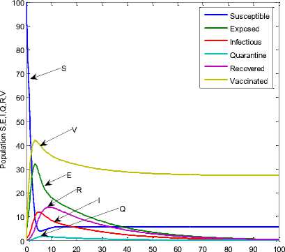
We present the numerical result using Runge-Kutta Fehlberg method of order 4 and 5. The network is assumed to have initial values: S=100; E=3; I=1; R=0; Q=0; V=0. Fig. 3 shows the behavior of susceptible, exposed, infectious, recovered, quarantine and vaccination class with respect to time. From Fig. 3 we observed that the system is asymptotically stable.

Time in minutes

Fig. 3: Dynamical behavior of the system for different classes when

Λ =.1; β=.1; σ=0.3;d=0.003;φ=.4; ε=0.3;

ρ=0.06;γ=0.3;α=.1;δ=0.2; η =0.4

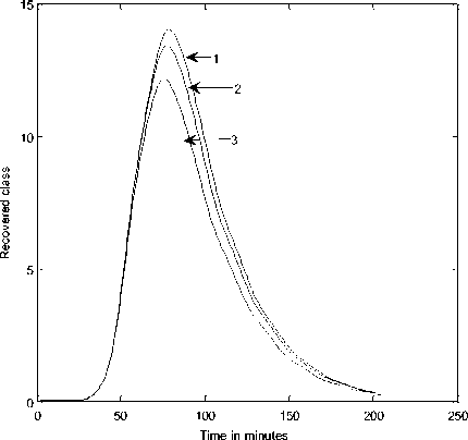
Fig. 5: Dynamical behavior of recovered class with respect to time

(1) Λ =.1; β=.1; σ=0.3;d=0.003;φ=.4; ε=0.3;

ρ=0.06;γ=0.3;α=.1;δ=0.2; η =0.4

(2) Λ =.1; β=.1; σ=0.3;d=0.003;φ=.43; ε=0.33;

ρ=0.06;γ=0.3;α=.1;δ=0.2; η =0.4

(3) Λ =.1; β=.1; σ=0.3;d=0.003;φ=.46; ε=0.39;

ρ=0.06;γ=0.3;α=.1;δ=0.2; η =0.4

Fig. 3 shows a powerful impact of vaccination class over exposed, infectious and quarantine class. As expected, over time I(t) first increases gradually as the R(t) capacity increases the infection become smaller. Fig. 4 shows V(t) class, if parameters are well taken into account, we observe the impact of vaccination will be strong. Fig. 5 shows the analysis of R(t) class we observe the recovery rate is very high under different setting of parameter.

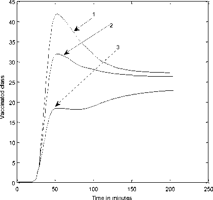
Fig. 4: Dynamical behavior of vaccination class with respect to time

(1) Λ =.1; β=.1; σ=0.3;d=0.003;φ=.4; ε=0.3;

ρ=0.06;γ=0.3;α=.1;δ=0.2; η =0.4;

(2) Λ =.1; β=.1; σ=0.2;d=0.003;φ=.4; ε=0.3;

ρ=0.04;γ=0.3;α=.1;δ=0.2; η =0.4;

(3) Λ =.1; β=.1; σ=0.1;d=0.003;φ=.4; ε=0.3;

ρ=0.02;γ=0.3;α=.1;δ=0.2; η =0.4;

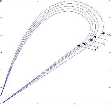
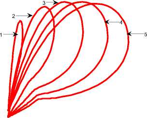
Fig. 6 shows the relationship between of I(t) and R(t) class under different setting of parameters, we observe from the fig. 6 that the recovery is very high. The effect of Q(t) is observed on different classes as depicted in fig. 7. Quarantine plays an important role in the recovery of the nodes. The quarantine nodes are treated with anti-malicious software and kept under constant observation

Infectious class

Fig. 6: Dynamical behavior of recovered class versus infectious class

(1) Λ =.1; β=.1; σ=0.3;d=0.003;φ=.4; ε=0.3;

ρ=0.06;γ=0.3;α=.1;δ=0.2; η =0.4,

(2) Λ =.1; β=.1; σ=0.3;d=0.003;φ=.42; ε=0.33;

ρ=0.06;γ=0.3;α=.1;δ=0.2; η =0.4,

(3) Λ =.1; β=.1; σ=0.3;d=0.003;φ=.44; ε=0.35; ρ=0.06;γ=0.3;α=.1;δ=0.2; η =0.4,

(4) Λ =.1; β=.1; σ=0.3;d=0.003;φ=.46; ε=0.37; ρ=0.06;γ=0.3;α=.1;δ=0.2; η =0.4,

(5) Λ =.1; β=.1; σ=0.3;d=0.003;φ=.48; ε=0.39; ρ=0.06;γ=0.3;α=.1;δ=0.2; η =0.4,

(3) Λ =.1; β=.1; σ=0.3;d=0.003;φ=.4; ε=0.7;

ρ=0.06;γ=0.3;α=.1;δ=0.2; η =0.8

(4) Λ =.1; β=.1; σ=0.3;d=0.003;φ=.4; ε=0.9;

ρ=0.06;γ=0.3;α=.1;δ=0.2; η =1

(5) Λ =.1; β=.1; σ=0.3;d=0.003;φ=.4; ε=1.1.;

ρ=0.06;γ=0.3;α=.1;δ=0.2; η =1.2

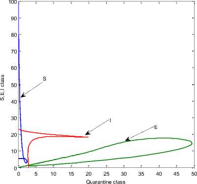
Fig. 7: Effect of Qarantine class on different classes when

О

-5

-5

Λ =.1; β=.1; σ=0.3;d=0.003;φ=.4; ε=0.3;

ρ=0.06;γ=0.3;α=.1;δ=0.2; η =0.4

Fig. 8 shows the effect of Q(t) and R(t) class under different setting of parameter. As the quarantine rate increases R(t) rate increases quickly. Fig. 9: shows the relation between Q(t) over I(t) class. When the nodes are highly infected by different malicious objects, quarantine is one of the remedy.

Quarantine class

Fig. 8: Dynamical behavior of quarantine vs recovered class

(1) Λ =.1; β=.1; σ=0.3;d=0.003;φ=.4; ε=0.3;

ρ=0.06;γ=0.3;α=.1;δ=0.2; η =0.4

(2) Λ =.1; β=.1; σ=0.3;d=0.003;φ=.4; ε=0.5;

ρ=0.06;γ=0.3;α=.1;δ=0.2; η =0.6

Infectious class

Fig. 9: Dynamical behavior of Infectious vs quarantine class

(1) Λ =.1; β=.1; σ=0.3;d=0.003;φ=.4; ε=0.3;

ρ=0.06;γ=0.3;α=.1;δ=0.2; η =0.4

(2) Λ =.1; β=.1; σ=0.3;d=0.003;φ=.4; ε=0.3;

ρ=0.06;γ=0.5;α=.3;δ=0.2; η =0.4

(3) Λ =.1; β=.1; σ=0.3;d=0.003;φ=.4; ε=0.3;

ρ=0.06;γ=0.7;α=.5;δ=0.2; η =0.4

(4) Λ =.1; β=.1; σ=0.3;d=0.003;φ=.4; ε=0.3;

ρ=0.06;γ=0.9;α=.7;δ=0.2; η =0.4

(5) Λ =.1; β=.1; σ=0.3;d=0.003;φ=.4; ε=0.3;

ρ=0.06;γ=1.1;α=.9;δ=0.2; η =0.4

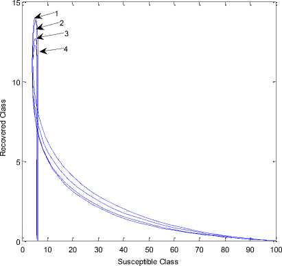
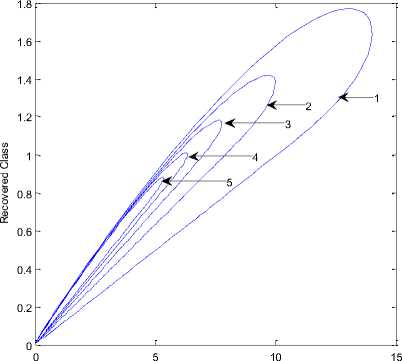
Fig. 10: Dynamical behavior of the recovered vs susceptible classes when

(1) Л =.1; в=.1; □=0.3;d=0.003;ф=.4; е=0.3;

ρ=0.06;γ=0.3;α=.1;δ=0.2; η =0.4,

(2) Λ =.1; β=.1; σ=0.3;d=0.003;φ=.4; ε=0.3;

ρ=0.06;γ=0.3;α=.1;δ=0.2; η =0.4

(3) Λ =.1; β=.1; σ=0.3;d=0.003;φ=.4; ε=0.3;

ρ=0.06;γ=0.3;α=.1;δ=0.2; η =0.4

(4) Λ =.1; β=.1; σ=0.3;d=0.003;φ=.4; ε=0.3;

ρ=0.06;γ=0.3;α=.1;δ=0.2; η =0.4

Fig. 10 shows the transfer of nodes from R(t) to S(t) class. As time passes, S(t) decreases gradually to zero. Which does not imply network failure; it implies that as the recovery rate increases the susceptibility towards infection decreases. The dynamical behavior of vaccinated class of nodes versus susceptible class of nodes is depicted in figure 11. As the rate of vaccination increase the susceptibility towards the attack of worm decreases.

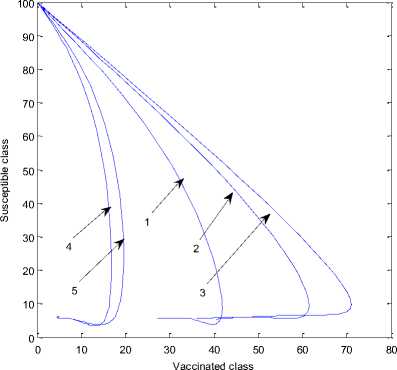
Fig. 11: Dynamical behavior of vaccinated class vs susceptible class when

(1) Λ =.1; β=.1; σ=0.3;d=0.003;φ=.4; ε=0.3;

ρ=0.06;γ=0.3;α=.1;δ=0.2; η =0.4

(2) Λ =.1; β=.1; σ=0.6;d=0.003;φ=.4; ε=0.3;

ρ=0.09;γ=0.3;α=.1;δ=0.2; η =0.4

(3) Λ =.1; β=.1; σ=0.9;d=0.003;φ=.4; ε=0.3;

ρ=0.12;γ=0.3;α=.1;δ=0.2; η =0.4

(4) Λ =.1; β=.1; σ=0.12;d=0.003;φ=.4; ε=0.3;

ρ=0.15;γ=0.3;α=.1;δ=0.2; η =0.4

• IV.    Conclusion

The proposed SEIQRS-V model captures both the spatial and temporal dynamics of worms spread process. Reproduction number (R 0 ), equilibria, and their stability are also found. If R 0 <1 the worm free equilibrium (E 0 ) is globally stable in the feasible region and the disease always dies out. If R 0 >1, a unique endemic equilibrium E^*  exists and is locally asymptotically stable.

Verification and validation of our model parameter has been analyzed by simulating the system. The model addresses the worm containment based on the dynamic quarantine on the node in a group that has exhibited highly infectious behavior. By Quarantine we achieve fast recovery and end the susceptibility of spread of infection to benign nodes. By vaccinating the nodes in a group immunized them toward the infection and enabling guideline for typical active worm control. The study will be helpful to the software organization in developing efficient antivirus for sensor network.