Density based initialization method for k-means clustering algorithm

Published Online October 2017 in MECS

Data clustering is an unsupervised learning process used to partition n objects in a pre-defined k groups in such a way that objects within the groups are similar to each other than those in other groups [1]. Clustering algorithms are used in a variety of scientific areas, including bigdata [2], image processing [3-4], GIS application [5], business intelligence [6], market analysis social networks [7], anomaly detection [8], and security [9].

Numerous clustering approaches has been documented in the literature such as hierarchical [10], partitioning, density-based [11], model-based and grid-based [12]. In the partitioning technique given data set is divided into k groups (k < n, n is the size of the data set). Due to simplicity, computational speed and easy to implement k-means algorithm is the preferred choice among partitioning algorithms [13].

The k-means clustering algorithm finds the groups in the data set by minimizing an objective function [14]. For the dataset X={X 1 , X 2 ,…..,X n } with n observations, the purpose of k-means clustering is to find k groups in X as C={C₁,C₂,…C_k} such that the objective function f_km is minimized:

nk

fm =XXz^r ^     (1)

i = 1 k = 1

Where Z ik is a variable defined in “(2)”.

z = 11   if Xie Ck ik   I 0 therwise

C_k represents the k^th cluster and μ_k represents the mean vector of the observation C_k.

The k-means algorithm provides a locally optimized solution [1]. It uses a set of randomly chosen initial seed value as centers and repeatedly assigns the input data points to a cluster based on distance to initially selected centers. The algorithm continues until the cluster mean no longer changes in the successive step. The k-means algorithm stops when the class label of the data points at i^th iteration is identical to i+1.

The main advantage of k-means algorithm is that it always finds a local optimum for any initial centroid locations. Despite being used in an array of application, the k-means algorithm is not exempt from limitations. From a practical point of view, the seed value of the algorithm is vital since each seed can produce different local optima leading to varying partitions. The quality and efficiency of the algorithm can vary far away from the global optimum, even under the repeated random initialization. Therefore, good initialization is critical for finding the optimal partitions. Several methods are documented in the literature on improving the initialization procedure that changes the performance, both in terms of quality and convergence properties [15]. In addition, various validity measures are also indexed in the literature for the comparison of perfectly partitioned results [1].

The rest of the paper is framed as follows. Section 2, we include a brief survey of the existing work on cluster center initialization for the k-mean algorithm. The proposed kernel density-based method to compute the initial seed value of k-means clustering algorithm is presented in Section 3. Whereas, in Section 4, detailed experimental analysis of the proposed method and comparison of the result is shown. Finally, Section-5 concludes the work presented in this paper with pointers to the future work.

• II.    Related Work

The k-means method requires random selection of initial cluster centers. As discussed earlier, an arbitrary choice of initial cluster centers leads to non-repeatable clustering results that may be difficult to comprehend. The results of partitional clustering algorithms are better when the initial partitions are close to the final solution [10]. A short review of the existing work is included in this section for computing an initial seed value of a k-means clustering algorithm.

Bradley and Fayyad in 1998 documented a refinement algorithm that builds a set of small random sub-sample of the data and then performed clustering in each subsample by k-means [16]. The centroid of each sub-sample is afterward clustered together by k-means using the k-centroid of each sub-sample as an initial center. Likas et al. in 2003, introduced the global k-means algorithm, which performed an incremental clustering by adding one cluster center at a time through a deterministic global search procedure comprising N (with N being the size of data set) executions of k-means algorithm from the suitable initial positions [17].

Khan and Ahmad in 2004 presented the cluster center initialization algorithm (CCIA) to solve the cluster initialization problem [18]. The CCIA algorithm uses k-means and density based multi-scale data condensation method to separate the data into a suitable partition. Mirkin in 2005 presented a “Max-Min” algorithm for initialization. It tries to find initial seed value of the real observations that are well separated from each other [19]. Deelers and Auwantanamongkol in 2007 documented an algorithm to compute initial centers for k-means algorithm [20]. In this work, a cutting plane is used to separate the dataset into a smaller cell. The plane is used to reduce the sum of squared error of the two cells and find the cells that are far apart as possible to the data axis with the highest variance. Arthur and Vassilvitskii in 2007 introduced k-means++ algorithm to find initial consecutive centers with probability proportional to the distance to the nearest center [21]. The algorithm appraises the initial seed selection based on the sum of the square differences between a member of cluster and the cluster center which is normalized to the data size.

Belal and Daoud in 2007 developed an algorithm to initialize the k-mean algorithm [22]. First, the dimension with maximum variance is selected and then the attribute is sorted after that it is divided into a set of groups. The median for each group is used to initialize the k-means. Maitra in 2009 used local modes present in the data set to initialize the k-means algorithm [23].

Murat et al. in 2010 introduced a new method of cluster center initialization [24]. This method used to find two variables that best described the changes in the data set. Khan in 2012 introduced a simple initial seed selection algorithm for k-means clustering along one attribute that draws initial cluster boundaries along the deepest valleys or greatest gap in the data set [25]. It incorporates a measure to maximize a distance between the consecutive cluster center, which augments the conventional k-means optimization for minimum distance between a cluster center and cluster members. Malinen et al. in 2014, developed a new algorithm k-means*, an opposite approach to traditional approach. The method performs local fine-tuning of a clustering model of pathological data having the same dimension to the given dataset [26].

Many kernel based approaches have been used for solving the clustering problem. Piciarelli et al. in 2008 developed a data clustering technique when there is no prior knowledge about the number of cluster [27]. The method is inspired by SVM and uses feature space of Gaussian kernel for performing data clustering. In [25], the authors have developed a novel technique to detect the correct number of cluster by using the geometric properties of the normalized kernel space to predict the correct number of cluster [28].

The k-mean, k-means++, Fast global k-means and k-means* are used to show the effectiveness of the proposed algorithm. Some other algorithms are also used for checking the validity of the proposed algorithm on small datasets.

• III.    Proposed Algorithm

In this section, we first discuss the nearest and furthest point on a parametric curve, followed by density estimate and overview of the algorithm with naïve example and then present the Pseudo-code of the proposed algorithm.

• A.    Furthest Point on a Parametric Curve

Given a parametric curve C(t) =(x (t), y (t)) and a point A= (u, v) , the Euclidean distance between A and a point B on a parametric curve C(t) is defined by “(3)”.

d ( A,B ) = ( V ( u - * ( t)) 2 + ( v — У ( t )) 2 )           (3)

The local maximum and minimum value of “(3)” can be obtained by equating the differential of “(3)” to zero i.e.

d Г d ²( A, C ( t )) 1 = 0               (4)

dt

To find the nearest point on the C(t) from the given point A= (u, v), we have to consider the odd multiplicity roots of “(4)”, because only at those points the function Changes its sign. It has been shown in “Fig.1”.

The nearest distance of a parametric curve C(t) =(x (t), y (t)) from a given point is equivalent to “(5)”.

d ( A, C ) = min d ( A, C(t ))

Where I is the odd multiplicity roots of the polynomial, A(t)=(u-x(t)).xꞌ(t)+(v-y(t).yꞌ(t) .

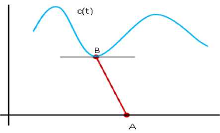
Fig.1. Distance from point A to a curve C (t).

Similarly, as shown in Fig.2, the farthest point on a parametric curve C(t) =(x (t), y (t)), t e I from A is a point C(t0), t0 e I such that, variable P than the kernel density estimate is a sum of n kernel functions. In this paper, the popular Gaussian kernel has been used to estimate the density.

Each Gaussian kernel function is centered on a sample data point with variance h, which is defined as bandwidth and it is used to control the level of smoothing. The density of the data points depends on the width of Gaussian kernel, so a proper value of h is obtained from the Silverman approximation rule [29] for which h = 1.06 x S | P | ^{( - 1/5)} where 5 is the standard deviation of the sample data points P . In one-dimensional case the density estimator is defined as follows:

^{P ( x} ) =

[ ^x - p ] ²

¹___V/ 2 h ²

^ e

For the d-dimensional case, the kernel function is the product of d Gaussian functions; each with its own bandwidth h j , henceforth, the density estimator is defined as follows:

Г x . D, - p . D , 1 ²

1                       d — ^L j 7 j ^J

P ( x ) =----- ,, Ш    ² h^j      (8)

I P I [ 2 П ] 2 П j J '! ^{P e} " j "

d ( A , C (t ₀ )) = max d ( A , C (t ))           (6)

t e I

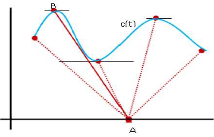
Fig.2. Farthest point B on a curve.

On the basis of above discussion, we present our algorithm to select an initial seed value for the k-means algorithm that has a high impact on the clustering results. Instead of random selection, the proposed method uses the density of the data points as a measure for finding K seed values. These data points are selected from the denser region of the data sets and furthest from each other.

• B.    Density Estimation and Overview of the Proposed Method

The kernel density [27] technique is employed here to estimate the probability density function of a continuous random variable. If X={X 1 , X 2 ,…..,X n } is a sample from a

Where a d-dimensional point p is denoted by {P.D 1 , P.D2,…, P.Dj} .

The algorithm starts by choosing the attribute value in a n×m data matrix, having largest variance. From the selected attribute value, we place a Gaussian kernel on each attribute value to estimate the final density estimate of the selected attribute and by using this estimate we select k initial center for the proposed method. The whole process is explained with the help of example.

Example: Consider a single dimensional artificial data set given in the Table 1, where {x1, x2,…, x10} are data points of an object X having largest variance in the given data matrix.

• Table 1. An artificial data set

  Object	x1	x2	x3	x4	x5	x6	x7	x8	x9	x10
  X	-1.08	0.03	0.55	1.1	1.54	0.08	-1.49	-0.74	-1.06	2.35

A Gaussian kernel is now placed over each data point of object X t o estimate the final density by using “(7)”, see Fig.3.

Further, by using the final density estimate and “(6)” the first center ‘ S1 ’ is selected, where density is maximum, see Fig.4.

Next, we compute the distances of each point on the curve from the ‘ S1 ’ by using “(9)”.

^D ( i , _s 1 ) =V ( x i - ⁵ 1 ) ² , i = ¹’²’-’ n          ⁽⁹⁾

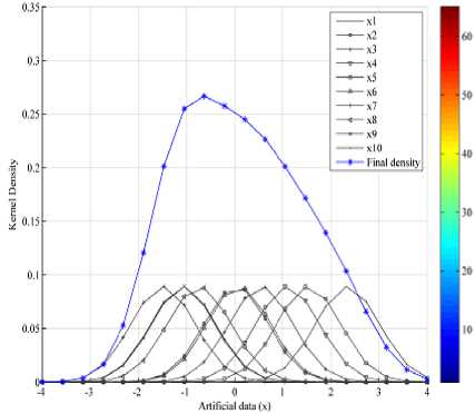
Fig.3. Computation of kernel density for one dimensional data

The data point with highest distance of D (i,s1 ) will be selected as second center. To select the next S j for the initial center, D (i,sj) (j is the current iteration) is calculated between each data points and previously computed centers S j _-1 . The data point with the highest value of sum of distance D ( _i,s j _-1 ) will be selected as next center, see Fig.5. For example the third seed value is the data point obtained by using “(10)”.

5 3 = max( D _{( /} ,^ + D ₍ , , s 2 ) )          (10)

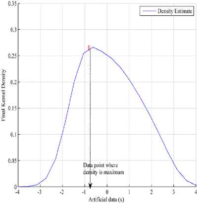
Fig.4. Computation of maximum density point from point A to a curve C(t).

The process continues selecting points in this way until the number of initial cluster centers equals to the predefined number of clusters.

The example describes how to choose the k initial cluster center. From the density estimate of the data points we will select first center where the density is maximum which is mark as s1 in Fig. 5. The other K-1 centers are selected from the data set that are at maximum distant from the first center (s1) and at maximum distant with respect to each other, see Fig. 5. These selected point’s s1, s2 and s3 are used for the initialization. The proposed scheme of initial center selection is briefly described in Algorithm 1.

Algorithm 1 : Initial-center ( X, k )

Input:   Dataset X = { Xj }    , the number of cluster k.

Output: A set of k initial center’s.

Procedure :  Initial-center ( X, k )

• 1:     P(x)^X // kernel density estimate of the dataset X

• 2:     for each data point x i ϵ X do

• 3:   d ( x , P ) = d ( X , P ( x ))

  // The Euclidean distance of //point from the curve

• 4:             S 1 ← max( d ( x , P ))

  // Selection of first initial center

Kernel Density                               Filial Kernel Density

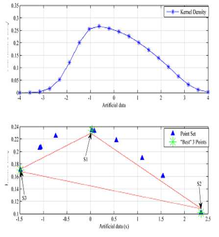
Fig.5. Selection of initial cluster center from the density curve.

• 5:                  D(i , 5 ) =>/ ( Xi - 5 ) 2 , i = 1,2,..., n

• 6:     S 2 ← max( D _{( i , s )} )

  // Selection of Second center

• 7:     For every other center do

• 8:                  ^Dis = ^D ( i , _Sj )

  //Distance between data points and previously computed center’s ( S j-1 )

• 9:                   S 3 = max ( D _{( i , s 1)} + D _{( i , s 2)} )

• 10:               S j =  (max ( D _{( i , s )} + D _{( i , s )}   +…+

^{D (} i . ⁵ j - 1 ) )

• 11:    if j=k (predefined center are selected) then

• 12:                Stop

• 13:      else

• 14:               Go to line 11.

The good thing about this method is that it can avoid the nearest data points to S J _{- 1} being chosen as the next initial cluster center. The furthest point selection strategy helps in spreading the initial center throughout the data set and helps k-means algorithm to converge with fewer iteration but in some cases when the size of data is small it tends to select outliers as center that is not a good candidate for initial center.

After selecting the initial centroid, the process of finding cluster is similar to the k-means algorithm. Now, with the help of algorithm 1, the clustering procedure is summarized by following steps:

Step 1. Normalize the data set X

Step 2. Find and select the attribute having maximum variance

Step 3. The density estimate at all the data points for the selected attribute by using the Gaussian window. For the multidimensional data the density is estimated by using “(8)”, where the kernel function is the product of d Gaussian function, each with its own bandwidth.

Step 4. The first center is chosen from the data points where the density is maximum. From the first center find the distance of all other points , and the next (k-1) probable center is chosen from the distance matrix where density is maximum provided that the sum of distances between these points are maximum.

Step 5. Using indices of the data points in the previous step selects k data points of the density value to be used for the initialization purpose.

Step 6. Execute k-means algorithm with the help of initial seed value computed in the previous step.

The motive behind the above method is to find initial points from the denser area of the dataset. In this way, the selected data points represent the common characteristics of the entire dataset and it is used for initialization.

In the next subsections, first, we compare the time complexity of the proposed approach with other existing method and then the short description of the validity measures used here to check the quality of the experimental results have been presented. We have used both internal and external validity measures, described in the literature for comparing the experimental results.

• C.    Time Complexity

The time complexity of the proposed algorithm is derived by the summation of complexity at different stages. These sub-phases are as follows:

• •    Normalize the dataset, t_x = О ( n )

• •    Attribute subset selection, t 2 = О ( n )

• •    Density estimation, the time complexity of kernel density estimation at k evaluation points for given n sample point, t ₃ = О ( nk )

• •    Selection of k points from density estimate step 4, complexity of binomial coefficient, c ( n , k ) choosing k objects from among n objects, t₄ = О ( nk ) .

• •    The complexity of k-means algorithm for fixed, i number of iteration, t_s = О ( inkd ) , where n is the size of given data set, d is the dimension and k is the number of cluster.

The overall time complexity of the proposed algorithm is T = t + t ₂ + t ₃ + t ₄ + t₅ = О ( inkd ) .

The proposed method is asymptotically equivalent to the k-mean algorithm and faster than the Global k-means algorithm, see Table 2.

Table 2. Comparison of time complexity

Algorithm	Time complexity
k-means	О ( k«n )
Global k-means	О ( k2 nn 2 )
Fast global k-means	О ( k2 n )
k-means*	О ( steps • k n ) )
Proposed	О ( inkd )

• D.    Evaluation Measure

Many validity measures are documented in the literature to check the quality of the clustering algorithm. It is important to evaluate the quality of a clustering algorithm because the result of various algorithms gives different clusters. Two types of clustering validation methods are used; one is internal validity measures and other is external validity measures. Internal validity measures test the intra-cluster similarity and inter-cluster dissimilarity based on the structure of the dataset whereas the external validation method uses a true label and computed label of the objects to evaluate the clusters [14].

The validity measures which are used to compare the quality of the proposed method have been described as follows:

• •    Mirkin (MI) : The Mirkin metric [30] is related to the number of disagreed pairs in the given sets. Mirkin metric is scaled in the interval [0, 1] which is 0 for identical sets of levels or complete finding of the pattern and positive otherwise.

• •    Adjusted Rand Index (ARI): It is one of the most popular external validation measures ranging from 0 to 1. A Higher value of ARI shows the better quality of clusters.

• •   MSE : The mean squared error MSE :

NM

^MSE = M TT d ( ^X i , j         (11)

• ^v i = 1 j = 1

• •    Dunn index : The Dunn's index measure is used to find the compactness of the data points within the cluster and cluster’s separation (minimum distance between clusters). The maximum value of the index represents the right partitioning.

• •    Davies-Bouldin index (DB) : The Davies-Bouldin criterion is based on a ratio of within-cluster and between-cluster distances [30].

The validity measures like RI, ARI, NMI and MI belongs to the external validity measure and MSE, Dunn and DB are in the internal measure.

• IV.    Experiment and Results

  We ran the proposed algorithm on several datasets. The datasets are taken from the UCI repository [31], and the summaries of their characteristics are given in the Table 3. The set s1, s2, s3 and s4 are artificial datasets consisting of Gaussian clusters with the same variance but increasing overlap. Some of these datasets can be found in the web page [23] https://cs.uef.fi/sipu/datasets as mentioned in the literature. In a1 and DIM datasets, the clusters are clearly separated whereas s1-s4 they are more overlapping. All the experiments are performed on Intel®Core™ i3-2348M machine with 2GB of RAM.

We have compared the result of the proposed method with seven existing methods indexed in the literature, see Table 4. Several runs of each algorithm have been performed, and most significant digits of the result are shown.

Table 3. Data Set description.

Dataset	Data Set Characteristics	Number of features	Number of data objects	Number of Clusters
Iris	Multivariate	4	150	3
Wine	Multivariate	13	178	3
Breast Cancer	Multivariate	31	569	2
Indian-Liver	Multivariate	10	583	2
Lung Cancer	Multivariate	56	32	3
Thyroid	Multivariate	5	215	3
WDBC	Multivariate	32	569	2
Yeast	Multivariate	9	1484	10
Glass	Multivariate	32	569	7
a1	Artificial	2	3000	20
Dim032	Artificial	32	1024	16
s1-s4	Artificial	2	5000	15

Table 4. Abbreviation used for implemented algorithms.

S.No	Author’s Name / Method	Abbreviation used
1	Random Method	k-means
2	Arthur, D and Vassilvitskii,2007	k-means++
3	Likas et al., 2003	Fast GKM
4	Belal, Moth'd and Daoud, 2007	k-median
5	Murat et al., 2010	Mix
6	Khan, Fouad., 2012	Gap
7	Malinen et al. in 2014	k-means*
8	Proposed Method	Proposed

First, we made a comparison of the proposed method with k-means and the k-means++ algorithm by using the two validity measure, MSE and Davies-Bouldin index (DB). The proposed method uses initial centroid from the denser region and hence minimizes the inner class dissimilarity. The MSE results show that the proposed method is better or equivalent in 11 out of the 13 datasets used, see Table 5 and Fig. 6. The DB results show that the proposed method is better in 9 datasets out of the 13 datasets with respect to the k-means. It is also found better in 7 datasets out of 13 datasets as compared to the k-means++, see Table 6. We observe that the proposed algorithm competes with k-means and k-means++ and fails sometimes due to statistical property of the dataset. The proposed algorithm works well in high as well as low dimensionality datasets. Furthermore, it is stated that a clustering algorithm cannot be better than other for every dataset [26].

Table 5. MSE for 13 datasets, averages over several (>=10) runs are used.

Datasets	k-means	k-mean++	Proposed
Iris (×103)	1.63	1.31	1.31
Wine (×103)	1.02	1.09	1.02
Breast Cancer (×103)	4.57	4.57	4.57
Indian-liver data set(×104)	1.39	1.46	1.39
Lung Cancer (×103)	2.93	2.94	2.91
Thyriod	2.69	2.7	2.7
Yeast	0.018	0.007	0.004
Glass	0.26	0.23	0.19
a1	3.1	2.25	3.35
S1(×109)	1.79	1.19	1.79
S2 (×109)	1.98	1.73	1.7
S3 (×109)	1.88	1.87	1.87
S4 (×109)	1.73	1.69	1.68

Table 6. Davies- Bouldin index (DB) index for different datasets, averages over several (>=10) runs are used.

Datasets	k-means	k-mean++	Proposed
Iris (×103)	7.5	4.69	4.63
Wine (×103)	4.96	5.55	4.96
Breast Cancer (×103)	8.12	8.12	8.12
Indian-liver data set(×103)	1.56	1.26	1.56
Lung Cancer	1.84	2.04	2.06
Thyriod	2.07	2.13	2.81
Yeast	1.11	1.45	1.06
Glass	0.82	0.46	0.5
a1	4.11	1.99	1.06
S1(×1014)	2.06	4.71	0.57
S2 (×1014)	1.91	2.11	3.91
S3 (×1014 )	4.01	3.21	2.14
S4 (×1014)	2.26	3.48	5.55

Further, the proposed method is compared with Fast GKM and k-means*, see Table 8. The proposed method performs better or equivalent 8 out of 13 cases with respect to Fast GKM and k-means*. We observe that the proposed initialization works well in small dimensionality dataset. We, therefore, recommend proposed initialization method for low-dimensional unknown distribution. For the high dimensional dataset k-means++ or k-means* type of initialization works best.

We have also calculated Dunn and NMI, to validate the clustering quality, see Table 7, 9. We observe that the proposed method performs well in 4 out of 9 datasets for Dunn index and 4 out of 6 in terms of NMI index.

The proposed algorithm is also compared to other initialization methods indexed in the literature, see Table 4. We have used various validity measures like adjusted rand index, error, mirkin index for comparison. We observe that the proposed algorithm performs better in 4 out of 5 datasets with respect to error index, 2 out of 5 in terms of mirkin index and 1 out of 4 times in terms of adjusted rand index, see Table 10-14.

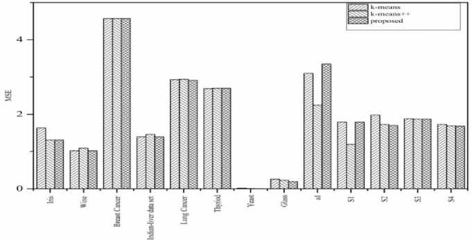
Fig.6. Comparison of mean square error (MSE) of the proposed algorithm with k-means and k-means++ on 13 datasets.

Table 7. Dunn index for 9 datasets, averages over several (>=10) runs are used.

Datasets	k-means	k-mean++	Proposed
Iris (×103)	1.24	1.68	1.69
Wine (×103)	1.5	1.01	1.5
Breast Cancer (×103)	2.01	2.01	2.01
Indian-liver data set(×103)	1.07	1.12	1.07
Lung Cancer	0.78	0.61	0.69
Thyriod	0.21	0.08	0.04
Yeast	0.04	0.01	0.36
Glass	0.11	1.06	0.59
a1	3.6	6.7	0

Table 8. MSE comparison with k-mean,k-mean++, Fast GKM and k-mean*, averages over several (>=10) runs are used.

Datasets	k-means	k-mean++	Fast GKM	k-means*	Proposed
Iris (×103)	1.63	1.31	2.02	2.42	1.31
Wine (×103)	1.02	1.09	0.88	1.93	1.02
Breast Cancer (×103)	4.57	4.57	-	-	4.57
Indianliver data set(×103)	1.39	1.46	-	-	1.39
Lung Cancer (×103)	2.93	2.94	-	-	2.91
Thyriod	2.69	2.7	1.52	6.96	2.7
Yeast	0.018	0.007	0.003	0.04	0.004
Glass	0.26	0.23	0.16	0.22	0.19
a1	3.1	2.25	2.02	2.38	3.35
S1(×109)	1.79	1.19	0.89	1.05	1.79
S2 (×109)	1.98	1.73	1.33	1.4	1.7
S3 (×109)	1.88	1.87	1.69	1.78	1.87
S4 (×109)	1.73	1.69	1.57	1.59	1.68

Table 9. NMI. Most significant index value of different datasets, averages over several (>=10) runs are shown.

Datasets	k-means	k-mean++	Proposed
Iris	0.7	0.75	0.76
Wine	0.43	0.42	0.43
Breast Cancer	0.46	0.46	0.46
Indian-liver data set	0.03	0.009	0.03
Lung Cancer	0.26	0.24	0.24
Thyriod	0.36	0.28	0.27

Table 10. Clustering results for Iris data.

Datasets	ERROR	RI	AR	MI	HI
k-means	0.18	0.8	0.6	0.2	0.7
k-means++	0.1	0.9	0.7	0.1	0.8
k-median	0.11	0.9	0.7	0.1	0.7
Mix	0.11	0.9	0.7	0.1	0.7
Gap	0.04	0.9	0.9	0.1	0.9
Proposed	0.1	0.9	0.7	0.1	0.8

Table 11. Clustering results for wine data set.

Datasets	ERROR	RI	AR	MI	HI
k-means	0.29	0.72	0.37	0.28	0.43
k-means++	0.31	0.7	0.36	0.29	0.40
k-median	0.2	0.77	0.49	0.22	0.54
Mix	0.2	0.77	0.49	0.22	0.54
Gap	0.2	0.77	0.49	0.22	0.54
Proposed	0.29	0.72	0.37	0.28	0.43

Table 12. Clustering results for Breast Cancer data set.

Datasets	ERROR	RI	AR	MI	HI
k-means	0.14	0.74	0.48	0.25	0.49
k-means++	0.14	0.74	0.48	0.25	0.49
K-median	0.24	0.62	0.23	0.37	0.25
Mix	0.37	0.53	0.13	0.46	0.06
Gap	0.37	0.53	0.13	0.46	0.06
Proposed	0.14	0.74	0.48	0.25	0.49

Table 13. Clustering results for Indian-liver data set.

Datasets	ERROR	RI	AR	MI	HI
k-means	0.28	0.56	0.02	0.43	0.13
k-means++	0.28	0.58	0.04	0.41	0.17
k-median	0.28	0.56	0.02	0.43	0.13
Mix	0.28	0.59	0	0.4	0.18
Gap	0.28	0.59	0	0.4	0.18
Proposed	0.28	0.56	0.02	0.43	0.13

Table 14. Clustering results for Lung Cancer data set.

Dataset	ERROR	RI	AR	MI	HI
k-means	0.43	0.6	0.14	0.39	0.2
k-means++	0.43	0.59	0.13	0.4	0.18
k-median	0.59	0.32	0	0.67	0.35
Mix	0.56	0.45	0.02	0.54	0.09
Gap	0.53	0.58	0.04	0.41	0.16
Proposed	0.43	0.62	0.13	0.37	0.25

Clustering algorithm cannot be guaranteed to be better than other in every case. In real-world application, k-means is often applied by repeating it several times starting from different random initializations and the best solution is kept finally. In clustering the main aim is to minimize inner class dissimilarity and maximize intraclass similarity. The reason, the methods work well is that initial seed values are obtained from the denser region of datasets and thus useful in minimizing inner class similarity. Furthermore, these points are at maximum distant from each other, helps in maximizing intra-class similarity.

• V.    Conclusiions

A novel kernel-based algorithm for initializing the k-means clustering algorithm is proposed in this work. Seven recent seed selection methods that cover a wide variety of initialization strategies are used for comparison of the results. The list does not include every possible strategy proposed in the literature. Indeed, it is not practical to compare every method available. However, the work provides a starting point in refining and evaluating new seed selection strategies for the k-means algorithm.

A set of initial seed value has been generated by estimating the density at each data point. A kernel is placed over the data point for selected dimension. Data points along with their density estimate are stored in another variable. Now, k points are selected from the stored variable in such a way that the first point is selected from the highest density estimate, and next k-1 points are selected such that points are at maximum distant from each other. Initial k density estimate is used for the initializing purpose. The proposed algorithm is simple to implement and has been tested on different benchmark data sets. Unlike k-means++ and k-mean* the proposed algorithm does not set up any new variables within the analysis. The proposed method improves the reproducibility of cluster assignments over different runs; a positive case since k-means produces different results at each run. The algorithm has applications in all areas of data analysis where a high level of replicability may be needed. In the area of Image segmentation, color reduction, computer vision and GIS application, the method can be used to standardize clustering results. The future work is how to find the width of a kernel for estimating the density.

• [1]    A. K. Jain and R.C. Dubes, “Algorithms for clustering data,” Prentice Hall, 1988.

• [2]    A. Kumar and S. Kumar, “Experimental Analysis of Sequential Clustering Algorithm on Big Data,” The IIOABJ, 2016, Vol.7 (11), pp. 160-170.

• [3]    Hamed Shah-Hosseini, “Multilevel Thresholding for Image Segmentation using the Galaxy-based Search Algorithm,” I.J. Intelligent Systems and Applications, 2013, 11, 19-33.

• [4]    A. Kumar and S. Kumar, “Color Image Segmentation via Improved K-means Algorithm”, International Journal of Advanced Computer Science and Application , 2016, Vol.7, No.3, pp. 46-53.

• [5]    E. Hadavandi, S. Hassan and G. Arash, “Integration of genetic fuzzy systems and artificial neural networks for stock price forecasting,” Knowledge-Based System , 2010, pp. 800-808.

• [6]    M. M. Rahman, “Mining social data to extract intellectual knowledge,” IJISA, 2012, Vol.4, no.10, pp. 15-24.

• [7]    A. Kumar, S. Kumar and S. Saxena, “An efficient approach for incremental association rule mining through histogram matching technique,” International journal of information retrieval research,” 2012, 2(2), pp.29-42.

• [8]    S. Kalyani and K. Swarup, “Particle swarm optimization based K-means clustering approach for security assessment in power system,” Expert System with Applications, 2011, Vol. 38, pp. 10839-10846.

• [9]    F. Murtagh and P. Contreras, “Algorithms for hierarchical clustering: an overview,” WIREs Data Mining Knowledge Discovery, 2012, Vol. 2, pp. 86-97.

• [10]    J. Sander, M. Ester, H.P. Kriegel and X. Xu, “Densitybased clustering in spatial databases: the algorithm GDBSCAN and its application,” Data Mining and Knowledge Discovery, 1998, Vol. 2, pp. 169-194.

• [11]    L. Kaufman and P. J. Rousseeuw, “Finding Groups in Data,” John Wiley & Sons, 1983.

• [12]    Y. Xiao and J. Yu, “Partitive clustering (K-means family),” WIREs Data Mining Knowledge Discovery, 2012, Vol. 2, pp. 209-225.

• [13]    D. Arthur and S. Vassilvitskii, “K-means++: the advantages of careful seeding,” In: Proceedings of the 18th Annual ACM-SIAM Symposium on Discrete algorithms, Philadelphia, PA: Society for Industrial and Applied Mathematics, 2007, pp. 1027–1035.

• [14]    P. S. Bradley and U.M. Fayyad, “Refining initial points for K-means clustering,” In: Proceedings of the 15th International Conference on Machine Learning, San Francisco, CA: Morgan Kaufmann, 1998, pp. 91–99.

• [15]    A. Likas, N. Vlassis and J. Jakob, “The global k-means,” Pattern Recognition, 2003, Vol. 36, pp. 451-461.

• [16]    S. S. Khan and A. Ahmad, “Cluster center initialization algorithm for K-means clustering,” Patter Recognition Letter, 2004, Vol. 25, pp.1293–1302.

• [17]    B. Mirkin, “Clustering for data mining: A data recovery approach,” Chapman and Hall, 2005.

• [18]    S. Deelers and S. Auwantanamongkol, “Enhancing K-means algorithm with initial cluster centers derived from data partitioning along the data axis with the highest variance,” International Journal of Electrical and Computer Science, 2007, Vol. 2, pp. 247-252.

• [19]    M. Belal and A. Daoud, “A New algorithm for Cluster Initialization,” World Academy of Science, Engineering and Technology, 2007, Vol. 4, pp. 568-570.

• [20]    R. Maitra, “Initializing partition-optimization algorithm,” IEEE/ACM Transactions on Computational Biology and Bioinformatics, 2009, Vol. 6, pp. 144-157.

• [21]    E. Murat, C. Nazif and S. Sadullah, “A new algorithm for initial cluster centers in k-means algorithm,” Pattern Recognition Letters, 2010, Vol. 32, pp. 1701-1705.

• [22]    F. Khan, “An initial seed selection algorithm for k-means clustering of georeferenced data to improve replicability of cluster assignments for mapping application,” Applied Soft Computing, 2012, Vol.12, pp. 3698-3700.

• [23]    M. I. Radu, R. Mariescu-Istodor and F. Pasi, “K-means*: Clustering by gradual data transformation,” Pattern Recognition, 2014, Vol. 47, pp. 3376-3386.

• [24]    C. Piciarelli, C. Micheloni and G. L. Foresti, “Kernelbased clustering,” Electronics Letters, 2013, Vol. 49, pp. 113-114.

• [25]    C. Piciarelli, C. Micheloni and G.l. Foresti, “Kernel-based unsupervised trajectory clusters discovery,” In: 8th International Workshop on Visual Surveillance, In conjunction with ECCV'08, France, October 17, 2008.

• [26]    H. Läuter and B.W. Silverman, “Density Estimation for Statistics and Data Analysis," Chapman & Hall, New York, 1986.

• [27]    R. M. Aliguliyev, “Performance evaluation of densitybased clustering methods,” Information Sciences, 2009, Vol. 179, pp. 3583-3602.

• [28]    B. Mirkin, “Mathematical Classification and clustering,” Springer, 1996.

• [29]    J. Qiao and Y. Lu, “A new algorithm for choosing initial cluster centers for k-means,” In: Proceedings of the 2nd International Conference on Computer Science and Electronics Engineering, 2013.

• [30]    K.Y. Yeung and W. L. Ruzzo, “An empirical study on principal component analysis for clustering gene expression data,” Bioinformatics, 2001, Vol. 17, pp. 763774.

• [31]    UC Irvine Machine Learning Data Set Repository, http://archive.ics.uci.edu/ml/datasets.html (accessed Jan 2016)

  
  
  

  Shishir Kumar has completed his Ph. D. (Computer Science) in 2005. He is working as Professor in Jaypee University of Engineering & Technology, Guna, India. He has sixteen years of teaching and research experience.

10.5815/ijisa.2017.10.05