Design and Comparative Assessment of State Feedback Controllers for Position Control of 8692 DC Servomotor

Published Online August 2015 in MECS

In industrial automation, the control of motion is a fundamental technological concern. Placing an object in the correct place with the right amount of force and torque at the right time is essential for efficient manufacturing operation [1]. Servomotor is a very vital electromechanical device used in providing a precise motion control, either linear or rotary motion. The basic reasons for using servo systems in contrast to open loop systems include the need to improve transient response times, reduce the steady state errors and reduce the sensitivity to load parameters [2]. Improving the transient response time generally means increasing the system bandwidth. Faster response times mean quicker settling allowing for higher machine throughput. Reducing the steady state errors relates to servo system accuracy.

Consider a simple pick and place robot shown in Fig.1. The robotic machine is used in an industrial set up to pick an object from one place (i.e point P) and place in another place (i.e point Q). The three joints of the robotic arm are made of servomotors. The angular position of each and every joint to complete this task of pick and place must be correctly determined [3] and controlled.

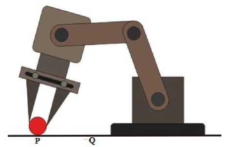
Fig. 1. Simple Pick and Place Robotic arm [3]

Over the years, little work have been carried out to compare the control performance of state feedback controllers for position control of dc servomotors. However, a huge step was taken in recent time by [4] to compare the control performances for position control using only full state feedback controllers and integral controllers.

This paper, however, investigates the performance of three different state feedback controllers (i.e full state feedback controller, full state feedback controller with feed forward gain and integral controller) in position control of Pittman dc servo motor. In other to achieve this, the state space mathematical model governing the behavior of the motor at any joint is undertaken. Controller design is carried out using pole assignment control technique via Ackerman’s formula [5] to determine the feedback gain matrix (K) and feed forward gain (N). Pole Placement design allows all closed loop poles to be placed in desirable locations [6]. Pole assignment has been considered because it has the best performance compared to other feedback controller design methods in terms of oscillation and settling time [7]. The pole placement design can also be used to study the control performance of linear time varying multiple input multiple output (MIMO) system [8]. The simulation results for stead state error, settling time and percentage overshoot were validated using MATLAB/SIMULINK software.

e_m (s) _

Kt

Uin^)   s[(L a S+R a )(/ m S+b m )+K_tK₆]

If armature circuit inductance L_a is neglected [10] and K_i = K _b — K for simplicity, then the transfer function of the armature controlled motor simplifies to (6).

⁶m(s) _      RgJm

Uin⁽s)    _s 2₊( ^Ra^bmVK²\

⁽ RgJm )

II. Mathematical Modeling of DC Servomotor

A. Electrical characteristics

Now, taking the inverse Laplace transform of (6) and manipulating yield (7)

®m

—

( ^^ ^b^)6₁ m +^U _i. (t)

KaJm         KaJm

The schematic diagram of armature controlled dc motor is given in Fig. 2.

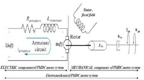
Fig. 2. Armature controlled DC servomotor [9]

Let the follows;

ia—

state variables of the actuator be assigned as

X ^ — ^m an d X 2 — ^m

—

1 e-Obm^ V   ^Ra^Jm

№ +

К

- RaJm-

Ui„ (t)

y ⁽ t) = [1

»i0

The general form of state space model for linear time invariant system (LTI) is given by (10) and (11) [11].

The torque T_M developed by the motor is proportional to the product of the armature current i _aand air gap flux ф^ assuming that the motor is operated over the linear region of the magnetization curve. T_m is expressed as in given in (1) where Ki is called the motor torque constant

Tm ® Vf ia — Kiia

The back EMF voltage, e_b induced in the armature windings is related to the motor shaft angular speed, w _m by a linear relation given by (2).

eb =Kb^ = KbWm(2)

Where 0m the servo is motor angular displacement and is back emf constant. The input voltage expression for the motor is given in (3).

Um (t) — L^ + R ai a + e b(3)

• B.    Mechanical characteristics

The torque, developed by motor produces an angular velocity, w _m , according to the inertia J _m and damping friction, b _m , of the motor and load. Performing energy balance on the motor system, the mechanical torque equation in differential equation form is given by (4) [9]. The equation has been considered for no load condition.

Jm^ + bm^=Tm = K i_a            (4)

• C.    State space model in continuous time

Transfer function given in (5) is obtained by taking the Laplace transform of (1), (2) and (3) and then eliminating armature current ( ) .

x(t) — Ax(t) + Bx(t) y(t) — Cx(t) + Dx(t)

Where;

A —

0 — (

^Ra^bm ^{+ K}

^Ra J m

■) B K I

/J I- R Jm!

C — [1  0] and D — 0

• III.    Controllers Design

In this section, we present the pole assignment technique via Ackerman’s formula for three different controllers and compare their performances in terms of percentage overshoot, settling time and steady state error.

• A. Full state feedback controller

The aim is to design a controller in the form: u = -Kx and to select coefficients of K in such a way that the eigenvalues of the closed loop system are placed in desired positions according to design specifications. The necessary and sufficient condition for placing the closed loop poles in arbitrary positions (i.e real eigenvalues and pairs of complex conjugate eigenvalues) is that the system is state controllable [6]. Fig. 3 illustrate a simple block diagram of full state feedback controller for any arbitrary plant. This controller is very simple in design, it also improves system characteristics such as rise time, settling time and overshoot but its major disadvantage is the large steady state error.

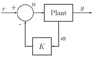
Fig. 3. General block diagram of full state feedback controller

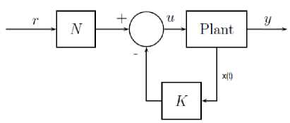
Fig. 4. State feedback controller with feed-forward gain for set point tracking

A more expanded form of control law is given in (12).

и(t) = -к _л x^t) - к ₂ x ₂(t) ----- k _u x _u(t) = -Kx(t) (12)

Where К = [кл k2......... kn] is a state feedback gain matrix. If this state feedback control law is connected to the system, the closed loop system is described by the state differential equation [6].

x(t) = (A - В)x(t)

Ackerman’s formula to evaluate the value of K is given as follows;

The state feedback is given by;

К = [0  0............. 1]M " ^((A)           (14)

Where;

M_c = Controllability matrix = [5 AB A ^{n— 2} В A ^n—гВ ]

a_c (Л) = M atrix p о lyn о m ia I

= A ⁿ + C n _— i_A ^{n 1} + ••• + C i A + ct₀1

= 0

The dominant poles to obtain the desired characteristic equation based on design specification is determined by evaluating the damping ratio ( ) and the un-damped natural frequency ( ) given by;

„ _   —In (POX 100)

^S     Vtt² + In (po OX 100)

Where;

= Settling time (sec); = Percentage overshoot

• B.    State feedback controller with feed-forward gain

State feedback controller with feed forward gain was introduced to eliminate the steady state error associated with full state feedback controller for any constant input as shown in Fig. 4. As an example, the control law is designed such that the output y(t) tracks the reference input r(t) i.e as t ^ ^, then y(Q ^ r(t). This controller achieves tracking only in the steady state when the reference inputs are step inputs. It does not achieve tracking when r(t) is changing rapidly. The gain K is outside the feedback loop and this makes the overall system to be sensitive to noise and disturbances. It is however, not ‘robust’ since any change in system parameter will cause non-zero error.

Suppose we let steady state vector xss = Nxr for any command input, then control law is defined as и =-K(x - xss) + uss(17)

Where is the steady state control effort to maintain x a.t xss. Also, let Nu and. Nb be defined by the following desired steady state relationships xss = A xss + В uss = (ANx + В Nu)r = 0(18)

yss = Cxss + D uss = (CNX + D Nu )r = r(19)

For all command input r, N_M an d N_x are determined as follows;

K]=[c Drill(20)

The compensated control law is now modified as и = -Kx + Nr(21)

Where N = N_M + N N_x

• C.    Integral controller with state feedback

Integral control technique is another kind of pole placement technique. It is also known as tracking controller as it required output to follow input command signal. The feedback from output is feedforwarded to the controlled plant via integrator. The integrator also known as integral action is used to increase the system type and reduce the previous finite error to zero [12]. The integral control technique configuration is shown in Fig. 5.

The introduction of the input integrator make the controller to have a pole at s = 0, thereby helping to get rid of the constant reference and thereby enhancing the robustness of the entire system. The design criteria involved in this controller is however more complex.

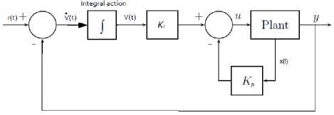
Fig. 5. Integral control with state feedback

The state feedback tracking controller is of the form:

и = -K_px + K_tv

Where;

Ki and K_p are integral gain and feedback matrix gain respectively.

Using this controller, the closed loop compensated system in state space representation becomes;

x А-B Kp   В Kt x 0

vJ   [-C + DKp  -D Kt\ LvJ + L1J'

The transfer function G(s) of the integral controller is obtained using;

G(s) = Ci[sI-Ai]-1Bi(24)

Where;

• - BKp   BKi0

Where; ^{A i} - ^[ —c + _DK^  -DK _t\ ; ^Bi = [0] ^and

C-[1 00]

• IV.    Simulation Results

  This section presents simulation results for three different feedback controllers for Pittman brush dc servomotor using Matlab/Simulink software. Comparative assessment between the three controllers and the command input is also presented. In other to examine the control performance of the state feedback controllers, the following design specifications were considered in all cases: System transient settling time (t_ss ) of 40ms and percentage overshoot of 16%. The physical parameters for Pittman 8692, 12Volt brush commutated dc servomotor is summarized in the Appendix A. Fig.6, Fig. 7 and Fig. 8 respectively illustrates the Simulink model diagrams of full state feedback controller, feed forward controller with state feedback (SFB) and integral controller with SFB.

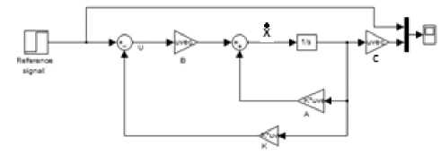
Fig. 6. Simulink model diagram of full state feedback controller

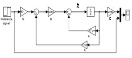
Fig. 7. Simulink model diagram of feed forward controller with SFB

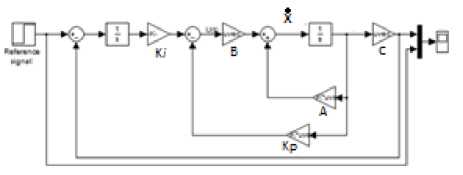
Fig. 8. Simulink model diagram of Integral controller with SFB

The simulation results for the full state feedback controller, feed forward controller with SFB, and integral controller with SFB are shown in Fig. 9, Fig. 10 and Fig. 11 respectively. Table 1 summarizes the simulation results of the three controller under normal operating conditions

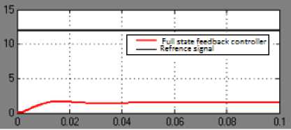
Fig. 9. Full state feedback controller

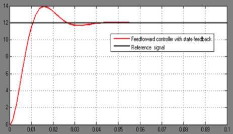
Fig. 10. Feed forward controller with state feedback

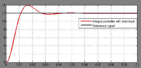
Fig. 11. Integral controller with state feedback

Table 1. Summary of the simulation results of the three controllers under normal operating conditions

Controller Types	Referenc e input (V)	Obtained. (V)	Steady state error (V)	Settling time (ms)	PO
Full state feedback	12	1.425	10.575	42	13.6
Feed forward gain with SFB	12	12	0	42.	13.7.
Integral with SFB	12	12	0	42	13.7

Meanwhile, in other to demonstrate the level of robustness between systems incorporating integral and the feed-forward controllers with state feedbacks, an external disturbance modelled by band limited white noise was introduced to corrupt the output of the plant as shown in Fig. 12.

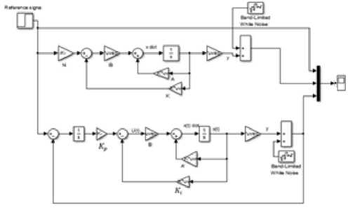
Fig. 12. Simulink model of feed forward controller with SFB and Integral controller with SFB under noise induced operating condition.

The simulation result comparing the output responses of integral and the feed-forward controllers with state feedbacks under normal and noise operating conditions with reference input is shown in Fig. 13. Table 2 summarizes the simulation results of these two controllers under noise operating conditions.

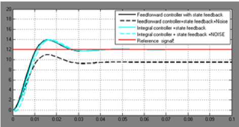
Fig. 13. Simulation result of feed forward controller with SFB and Integral controller with SFB under normal and noise induced operating conditions.

Table 2. Summary of the simulation results of feed forward controller with SFB and Integral controller with SFB under noise induced conditions.

Controller Types	Reference input (V)	Obtained. (V)	Steady State error (V)	Settling time (ms)	PO
Feed forward controller with SFB + Noise	12	9.4723	2.528	42	13.7
Integral controller with SFB + Noise	12	12	0	42	13.7

• V.    Discussions

The control performance of three different controllers have been analyzed in terms of maximum percentage overshoot, settling time and steady state error. In all circumstances, and within the limit of analytical error, the maximum percentage overshoot and settling time are the same and within the design specifications. However, in accurate positioning of object, it is desired that steady state error is zero. Thus, looking at the results given in table 1, it is clear that full state feedback controller is certainly not suitable for the industrial position control of object in proper location due to its very large steady state error. But comparing the feed forward controller with SFB and integral controller with SFB under normal operating conditions as show that the output responses really follow each other with feed forward controller a bit faster during the transient state.

Meanwhile, on injection of external disturbance signal in the output controlled variable of the plant as shown in fig. 12, a significant steady state error of about 2.53V is generated in the case of feed forward control while zero steady state error is still maintained in the case of feed forward controller. Based on this comparative results, it can be concluded that incorporating integral controller with state feedback in Pittman dc servomotor for position control is the best among the three controllers considered. Apart from being able to track the command signal, it is very robust and offers a very strict resistance to an external disturbing signal.

• VI.    Conclusions

In this paper, three state feedback controllers of the type full state-feedback controller, feedback controller with feed-forward gain and integral controller with state feedback have been designed to achieve position control of Pittman dc servomotor used in a simple pick and place robotic arm. The comparative assessment have shown that the three controllers exhibits similar behavior in terms of percentage overshoot and settling time under ideal situation. Full state feedback controller gave a very large steady state error compared to integral and feed forward controllers exhibiting zero tolerance to steady state errors. Under external disturbance condition, feed forward controller generate a significant steady state error while feed forward controller maintain the status of zero error. Based on the analysis, it can be concluded that integral controller is more robust and is therefore recommended for the precise position control.