Design of Fractional Order Recursive Digital Differintegrators using Different Approximation Techniques

Published Online February 2020 in MECS

Differintegrators is a term which is originated from the combination of differentiators and integrators together. Digital differentiators and integrators are two most important components of both integer order and fractional order calculus [1-21, 26]. These operators are the basic parts of many systems like signal processing, control, radar, sonar, communication, and medical applications. Integer order operators are useful for those systems which can be modeled using integral calculus. However, for various dynamic systems, integer order operators do not prove adequate to represent the characteristics accurately. For these types of systems, fractional order operators prove more useful as compared to the integer order ones [8-22].

The interest of these fractional order operators in signal processing applications have been motivated by their good performances and robustness in many applications. In addition, the generalization of derivatives and integrals from integer orders to fractional orders gives more flexibility in designing signal processing algorithms.

This paper focuses on Taylor series expansion (TSE) [11, 15], continued fraction expansion (CFE) [8, 14, 15, 16, 18], and rational Chebyshev approximation (RCA) [22, 23, 24, 25] based realization of a family of fractional order (α) differintegrators (FODIs) where α ∈ [0.1, 0.9] using Jain-Gupta-Jain second order integrator [3] by applying direct discretization method. The method using TSE and CFE expansion has been previously used by researchers in designing of FODIs for mostly α = 0.5. These are mainly based on first order operators and their results could not approximate the magnitude and phase characteristics of the ideal ones efficiently and even some of them have high computational complexity.

Rest of the paper is organized as follows. Section II presents the related works. Section III gives the problem formulation and solution methodology. Section IV presents the design of proposed FOIs and their comparison with the existing ones. Section V presents the proposed FODs and their comparison with the existing ones. The conclusions are given in section VI. Here, software MATLAB 8.0 is used to derive all simulation results and Nyquist frequency is taken as π radians/ second.

• II.    Related Works

In the literature, several definitions are given for arbitrary order differentiation and integration. The two most well-known definitions are the Riemann–Liouville (RL) and the Grunwald–Letnikov (GL).

RL definition (α > 0):

a Dft) =

1     dⁿ t    f( r )d r

Г(п - a) dtⁿ ' (t - T)^{a - n + 1}

where (n-1) < a < n and Г (х) represents the Gamma function of x.

GL definition (α ɛ R):

i   [ t ^- a /ho ]        (aA

D a f(t) = lim_h o .        £ ( - 1) ^aI - | ^f (t - kh o )

h₀ k = o       V ^k J

a i ₌       П а + ¹⁾                    (3)

k J  Г ( k + 1) Г ( а - k + 1)

where h 0 is time increment. As mentioned, the GL definition is valid for α > 0 (fractional differentiator) and for α < 0 (fractional integrator). From the perspective of control and signal processing applications, GL definition seems to be more useful, particularly in digital implementation.

One of important research topics of digital signal processing is to design digital fractional order differentiators (FODs) and fractional order integrators (FOIs).

The most popular methods are direct and indirect discretization using series expansion like continued fraction [8, 14, 15, 16], Taylor series [11, 15], and power series [12, 18], Pade’s approximations [9, 20], Prony’s approximations [9], Shank’s approximations [9], least squares approximations [10], weighted least square approximations [10], radial basis function [13], and impulse invariant discretization techniques [17]. In direct discretization method, a generating function is expanded by direct application of an expansion series. On the other hand, in indirect discretization method an efficiently fitted s domain rational approximation is discretized by using any existing s to z transformation.

• III.    Problem Formulation and Solution Methodologies

Integer order operators are useful for those systems which can be modeled using integral calculus. However, for various dynamic systems, integer order operators do not prove adequate to represent the characteristics accurately. It is well known that various existing lumped systems can be analyzed more accurately by fractional order systems as compared to the integer order ones. To effectively analyze complicated systems with fractional elements, it is necessary to develop approximations to the fractional operators using the standard integer order operators.

In literature, many algorithms have designed to improve the performance of digital FODIs. It is observed that getting efficient frequency response with low complexity is a difficult task.

In this paper, the main focus is to achieve efficiency of the ideal FODIs. For this, a family of new stable recursive FOIs is designed using three approximation techniques TSE, CFE, and RCA. Subsequently, by modifying the transfer function of FOIs appropriately, new stable FODs are obtained.

The order of the designed FODIs is basically an arrangement between the superior performance in frequency domain (obtained by increased number of coefficients) and better hardware implementation (obtained by lower number of coefficients). In this work, the maximum order of the resultant FODIs are restricted to five only.

• IV.    Proposed Fractional Order Integrators

In this Section, the transfer function of Jain-Gupta-Jain second order integrator [3] is expanded for fractional powers using three expansion methods like TSE, CFE, and RCA. Then, the approximated mathematical models are derived by collecting the coefficients of the numerator and denominator polynomials. It is expected to obtain the designed FODIs with better accuracy.

The design process can be summarized in the following two steps:

• (i)    Discretize the s- domain fractional order integrator using a suitable generating function (1/s)^α = (H(z^-1))^α where a denotes the fractional order, a e [0.1, 0.9].

• (ii)    Obtain the equivalent fractional order integrator, by performing TSE, CFE and RCA approximations over (H(z^-1))^α.

Here, expansion of (H(z-1))α is an infinite order of rational discrete-time transfer function. In this paper, the order of the approximate mathematical model of the fractional order integrators is taken as 5.

• A. Fractional Order Integrators via Taylor series expansion

A family of FOIs is designed using Jain-Gupta-Jain second order integrator H JGJ (z^-1) [3] and TSE. The transfer function of H JGJ (z^-1) (4) is taken as a generating function.

H jgj (z^-1) =

T (0.8647+ 0.5998z 1 +0.0541z ² ) (1-0.4812z ^-1 -0.5142z ^-2 )

So, the transfer function of FOIs for a e [0.1, 0.9] based on H JGJ (z^-1) can be expressed as:

(H JGJ (z^-1)) ^α = H ^α JGJ (z^-1)

T (0.8647 + 0.5998z^-1 + 0.0541z^-2) α

(1 - 0.4812z^-1-0.5142z^-2)

H TSE,0.9 ( z ^{- 1} ) =

0.8372(1+0.6243 z ^{- 1} +0.3469e-1 z ^{- 2}

+0.1599e-2 z ^{- 3} -0.6908e-3 z ^{- 4} +0.2731e-3 z ^{- 5} )

(1-0.4331 z ^{- 1} -0.4732 z ^{- 2} -0.2411e-1 z ^{- 3}

-0.1826e-1 z ^{- 4} -0.8422e-2 z ^{- 5} )

Clearly, (H JGJ (z^-1))^α is an infinite order of rational discrete-time transfer function. Here, MATLAB software is used to obtain the models of FOIs and series is truncated for fifth order polynomials (degree of the numerator and denominator is taken as 5).

The resultant transfer functions are unstable as poles are located outside the unit circle, these are stabilized by using pole reflection and magnitude compensation method suggested in [26]. After stabilization, the transfer function of the TSE deigned FOIs are shown as H TSE,α (z^-1) where α ∈ [0.1, 0.9], these are given in (6-14).

0.9697(1+0.6936e-1 z ^{- 1}-0.1539e-1 z ^{- 2}+ 0.5604e-2 z ^{- 3}-0.8238e-2 z ^{- 4}+0.1094e-2 z ^{- 5}) (6) (1-0.2548e-1 z ^{- 1}-0.6184e-1 z ^{- 2}-0.2544e-1 z ^{- 3} -0.1052e-1 z ^{- 4}-0.1603e-1 z ^{- 5})

H TSE,0.1 ( z  )

To define the efficiency of the designed FOIs, percentage absolute relative error (PARE) with respect to magnitude response is calculated in (15).

PARE ( ω ) =

^Mideal , α ^{( ω ) - M}TSE , α ^{( e - j ω )}

*100

^Mideal , α ^{( ω )}

Here, Mideal,α(ω)= ( jω)  = amplitude of the ideal fractional order (α) integrator          (16a)

MTSE,α(e-jω)= HTSE,α (z - )     = amplitude of the fractional order (α) integrator         (16b)

H TSE,0.2 ( z ^{- 1}) =

0.9450(1+0.1387 z ^{- 1}-0.2597e-1 z ^{- 2}

+0.1257e-2 z ^{- 3}-0.9357e-2 z ^{- 4}+0.1684e-2 z ^{- 5}) (7)

(1-0.9624e-1 z ^{- 1}-0.1214 z ^{- 2}-0.4494e-1 z ^{- 3}

-0.4010e-1 z ^{- 4}-0.2668e-1 z ^{- 5})

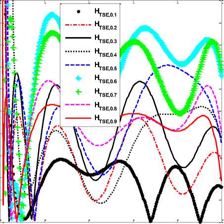
The PARE response of TSE designed FOIs is shown in Fig. 1.

H TSE,0.3 ( z ^{- 1} ) =

0.9187(1+0.2081 z ^{- 1}-0.3174e-1 z ^{- 2}

+0.0131e-1 z ^{- 3}-0.9543e-2 z ^{- 4}+0.1901 z ^{- 5})

(1-0.1444 z ^{- 1}-0.1786 z ^{- 2}-0.5859e-1 z ^{- 3}

-0.5117e-1 z ^{- 4}-0.3268e-1 z ^{- 5})

H TSE,0.4 ( z ^{- 1}) =

0.8903(1+0.2775 z ^{- 1}-0.3270e-1 z ^{- 2}

+0.0109e-1 z ^{- 3}-0.4318e-2 z ^{- 4}+0.1855e-2 z ^{- 5})

(1-0.1592 z ^{- 1}-0.1825 z ^{- 2}-0.4596e-1 z ^{- 3}

-0.3899e-1 z ^{- 4}-0.1434e-1 z ^{- 5})

H TSE,0.5 ( z ^{- 1}) =

0.8796(1+0.3468 z ^{- 1}-0.2884e-1 z ^{- 2}

+0.1000e-1 z ^{- 3}-0.3886e-2 z ^{- 4}+0.1636e-2 z ^{- 5}) (10)

(1-0.2406 z ^{- 1}-0.2598 z ^{- 2}-0.4768e-1 z ^{- 3}

-0.5747e-1 z ^{- 4}-0.13351e-1 z ^{- 5})

H TSE,0.6 ( z ^{- 1} )

0.8402(1+0.4001 z ^{- 1} -.0128e-1 z ^{- 2}

+0.8269e-2 z ^{- 3} -0.3189e-2 z ^{- 4} +0.1318e-2 z ^{- 5} ) (11)

(1-0.2887 z ^{- 1} -0.2830 z ^{- 2} -0.6562e-1 z ^{- 3}

-0.5353e-1 z ^{- 4} -0.2966e-1 z ^{- 5} )

ш8

7 о

ш

£5

<

О) з

0.2           0.4           0.6           0.8            1

Normalized Frequency (w/pi)

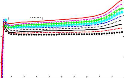
Fig.1. PARE response of TSE designed FOIs

H TSE,0.7 ( z ^{- 1})

0.8410(1+0.4856 z ^{- 1}-0.6701e-2 z ^{- 2}

+0.6067e-2 z ^{- 3}-0.9688e-2 z ^{- 4}+0.9575e-3 z ^{- 5}) (12)

(1-0.3368 z ^{- 1}-0.3843 z ^{- 2}-0.5703e-1 z ^{- 3}

-0.04542e-1 z ^{- 4}-0.2381e-1 z ^{- 5})

Group delay is a measure of phase distortion and it is calculated by differentiating phase with respect to frequency. The degree of nonlinearity of the phase indicates the deviation of the group delay from a constant.

H TSE,0.8 ( z ^{- 1} )

0.8359(1+0.5549 z ^{- 1} +0.1159e-1 z ^{- 2}

+0.3732e-2 z ^{- 3} -0.1496e-2 z ^{- 4} +0.5989e-3 z ^{- 5} ) (13) (1-0.3578 z ^{- 1} -0.4029 z ^{- 2} -0.4315e-1 z ^{- 3}

-0.3353e-1 z ^{- 4} -0.1654e-1 z ^{- 5} )

τ _g ( ω ) =

d θ ( ω )

d ω

Here phase of digital integrator is defined as θ(ω). The group delay response of proposed FOIs is shown in Fig. 2.

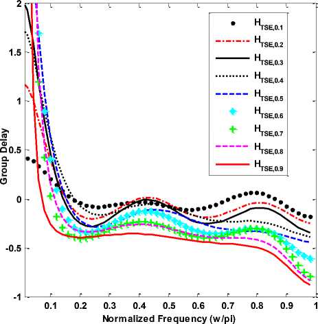
Fig.2. Group delay response of TSE designed FOIs

HCFE,0.3( z 1) = (

-0.9923-17.13 z ^{- 1} +106.05 z ^{- 2}

-24.82 z ^{- 3} -329.91 z ^{- 4} +269.3 4 z

1-43.58 z ^{- 1} +131.82 z ^{- 2} +68.15 z ~^-

-445.3 4 z ^{- 4} +291.41 z ^{- 5}

HCFE,0.4( z 1) = (

-0.6613-8.38 z “1 +62.33 z " ²

-22.05 z ^{- 3} -190.41 z ^{- 4} +165.62 z"

3)

.-5

1-29.88 z “1 +82.12 z ^{- 2} +54.09 z ^-:

-285.22 z ^{- 4} +180.52 z ^{- 5}

HCFE,0.5( z 1) = (

-0.5595-6.29 z ^{- 1} +44.14 z "²

-23.26 z ^{- 3} -12 3.61 z ^{- 4} +117.2 3 z"

3)

.-5

1-22.93 z ^{- 1} +57.39 z ^{- 2} +46.35 z ^-

-207.11 z ^{- 4} +126.2 5 z ^{- 5}

HCFE,0.6( z 1) = (

-0.549-2.3189 z ^{- 1} +27.93 z “²

-17.65 z ^{- 3} -88.05 z ^{- 4} +83.02 z

3)

.-5

1-18.71 z ^{- 1} +42.25 z ^{- 2} +41.30 z

-160.0 z ^{- 4} +95.15 z ^{- 5}

3)

B. Fractional Order Integrators via Continued fraction expansion

In the second technique, (H JGJ (z^-1))^α is expanded using CFE, and then depending on the order of the mathematical model required, the coefficients of the numerator and denominator polynomials are collected. In general, any function G(z) can be represented by continued fractions in the form of

HCFE,0.7( z 1) = (

-0.26101.45 z “1 +20.65 z ^{- 2}

-17.98 z ^{- 3} -61.21 z ^{- 4} +65.78 z

.-5

1-15.86 z ^{- 1} +33.08 z “2 +37.55 z

-129.03 z ^{- 4} +73.52 z ^{- 5}

3)

G ⁽ z) ~ a 0 ⁽ z) +

b ₁ ( z )

a 1 ⁽ z) +

b ₂( z )

a ( z ) +

b ₃ ( z )

a 3 ⁽ z ) + ..

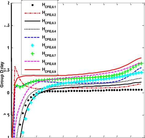
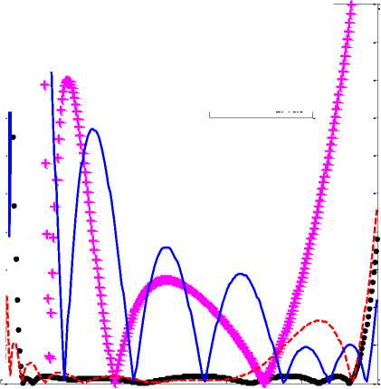
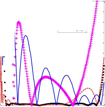
where the coefficients a i and b i are either rational functions of the variable z or constants. By truncation, an approximate rational function can be obtained. Here, transfer function of FOIs is obtained by collecting the coefficients of the numerator and the denominator polynomials for fifth order. The transfer function of CFE designed FOIs H CFE,α (z^-1) are given in (19-27). The PARE and group delay response of CFE designed FOIs are shown in Fig. 3 and 4, respectively.

-99.12-2018.12 z “1 +9306.23z - 2

H CFE,0.1

( z -1 ) = (

-0116.4S z ³ -2.87e4 z 4 +2.20e4 z 5 1-2753.65 z '■ 10220.11 ~²+2285.32 3

-32300.1 b "4 +23020.34 ^{- 5}

) (19)

-0.4467-45.11 z ^{- 1} +240.97 z “²

- 1      -33.56 z ^{- 3} -730.18 z ^{- 4} +590.97 z 5

H        (z ) = (-------Zi---------Z5--------ZT)  (20)

^CFE,0.²          1-83.59 z 1 +279.52 z ² +106.73 z ³

-910.17 z ^{- 4} +614.83 z ^{- 5}

^HCFE,0.8⁽ z 1 ) = (

HCFE,0.9( z 1) = (

-0.2920-36 z “1 +14.97 z ^{- 2}

-15.66 z “3-46.66 z “4+52.11 z"

- 5

1-13.81 z "1+2 6.31 z "2+34.74 z ^-

-107.52 z “4+59.53 z "⁵

-0.2398-0.0216 z ^{- 1} +11.52 z ^{- 2}

-14.07 z “3-34.97 z “4+42.97 z “⁵ x

1-12.2 6 z “1 +21.33 z “2 +32.50 z ^{- 3}

-91.68 z ^{- 4} +49.15 z ^{- 5}

Normalized Frequency (w/pi)

Fig.3. PARE response of CFE designed FOIs

1.5

0.5

-0.5

-1

0.1    0.2    0.3    0.4    0.5    0.6    0.7    0.8    0.9

Normalized Frequency (w/pi)

Fig.4. Group delay response of CFE designed FOIs

C. Fractional Order Integrators via Rational Chebyshev Approximation

In the third technique, (HJGJ(z-1))α is expanded using rational Chebyshev approximation (RCA), and then depending on the order of the mathematical model required, the coefficients of the numerator and denominator polynomials are collected. It is well known that Chebyshev polynomials provide approximations very close to the true continuous functions due to their fast convergence properties.

The integrator is first expanded for fractional powers.

If HPR,α(z-1) has no common polynomial factors in numerator and denominator, then there is a unique choice of p’s and q’s that minimizes λ; for this choice, λ(z-1) has (m+n+2) extrema in a ≤ z ≤ b, as mentioned by Ralston in [22]. Instead of making f(zi-1) and HPR,α(zi-1) equal at some (m+n+1) points zi-1, the residual λ(zi-1) can be forced to any desired value yi [23]. Remez algorithms [22, 24], based on Chebyshev polynomials theory, explain the process of convergence by an iterative process. Some of these algorithms are easily convertible to computer programs as suggested in [22, 25]. Here, we are using the algorithm proposed in [23] to find the optimal values of p’s and q’s. They provide the source code in C which can be easily used. Here, RCA is approximated in the interval [-0.9999, 0.9999] and degree of the numerator and denominator is taken as 5.

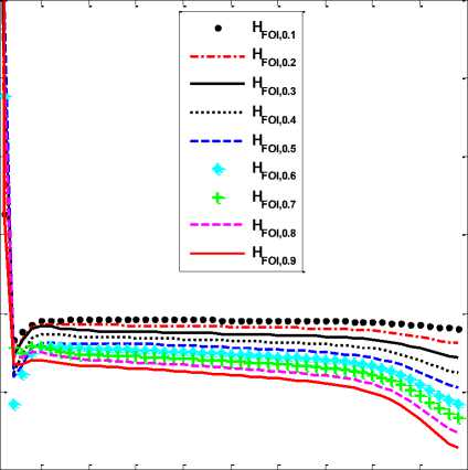
The transfer function of RCA designed FOIs are defined as HFOI,α(z-1), given in (31-39).

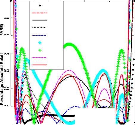
The PARE and group delay response of RCA designed FOIs are shown in Fig. 5 and 6, respectively.

-0.9867+1.2769z ^{- 1} + 0.0041 z ^{- 2}

-0.4146 z 3 +0.0885 z ~⁴+0.0023 z 5 x (31) 1.000(-1.4129 z ¹ + 0.1104 z 2 + 0.4400 z 3 -0.1185 z ^{- 4} + 0.000012 ^{- 5}

^HFOI,0.1^{( z}  ) = ⁽

-0.9724+1.2011 z ^{- 1} + 0.0554 z - 2

H FOI,0.2

( z ^{- 1}) = (

H FOI,0.3

(H jGj (z -1 )) ^e = f(z)              (28)

Let the desired rational function be H PR,α (z) which has a numerator of degree m and a denominator of degree n.

H PR _a (z -1 ) = ( ^p0 +_Р1г^4+р2^ ^{+ р}3^ ⁺...........................^{+ p}m^z"m ) , _f(z ^-1 )

,               ^{1 + q}1^{z + q}2^{z + q}3^{z +}........................... ^{+ q}n^z

Here, p 0, p 1, p 2,…. p m and q 1, q 2,…. q n are (m+n+1) unknown parameters. Let λ(z^-1) is the deviation of

H PR,r (z^-1) from f(z^-1), and λ is its maximum absolute value,

X(z ^-1 ) = H pR, a (z ^-1 ) - f(z ^-1 )       (30a)

X = max|X(z-1)|               (30b)

The ideal minimax solution would be that choice of p’s and q’s that minimizes λ. It is well known that finding a rational function approximation is not as straight forward as finding a polynomial approximation. The interval of approximation is considered as [ a , b ].

-0.3964 z ^{- 3} +0.0742 z 4 +0.0030 2 5 1.0000-1.4709 2 ^{- 1} + 0.1709 z 2 + 0.4473г ^{- 3}

-0.1338 z ^{- 4} + 0.0016 z ^{- 5}

-0.9563+1.1237 z ^{- 1} + 0.1028 z ^{- 2}

) (32)

( z ^{- 1}) = (

-0.3753 z 3 +0.0606 z 4 +0.0035 z ⁵

1.0000-1.5284 z ^{- 1} + 0.2339 z ² + 0.4524 z ^{- 3}

-0.1495 z ^{- 4} + 0.0034 z ^{- 5}

^HFOI,0.4^{( z} 1 ) = ⁽

H FOI,0.5

-0.9448+1.0542 z ^{- 1} + 0.1453 z ^{- 2}

-0.3562 z ^{- 3} +0.0487 z ~⁴ +0.0038 z - 5

1.0000-1.5854 z ^: ■ 0.2995 z ^-2 + 0.4549 z ^-3

-0.1655 z ^{- 4} + 0.0054 z ^{- 5}

-0.9311+0.9809 z ^{- 1} + 0.1851 z ^{- 2}

) (33)

) (34)

( z ^{- 1} ) = (

H FOI,0.6

-0.3337 z ~³ + 0.0362 z ~⁴ + 0.0041 z ^{- 5}

1.0000-1.6429 z 1 1 0.3680 z ^{- 2} + 0.4554 z ^{- 3}

-0.1817 z ^{- 4} + 0.0079 z ^{- 5}

-0.9187+0.9131 z ^{- 1} + 0.2204 z ^{- 2}

) (35)

( z —1 ) = (

H FOI,0.7

-0.3127 z ^{- 3} +0.0275 z ~⁴ +0.0039 z 5

1.0000-1.701 4z 1 1 0.4412 z ^-2 + 0.4525 z ^{- 3}

-0.1986 z ^{- 4} + 0.0106 z ^{- 5}

-0.9016+0.8405 z ^{- 1} + 0.2507 z ^{- 2}

) (36)

( z ^{- 1}) = (

H FOI,0.8

( z —1 ) = (

-0.2887 z ~³ + 0.0184 z ~⁴ + 0.0037 z 5

1.0000H.7552 z ^{- 1} + 0.5110 z ^-2 + 0.4500 z ^-3

-0.2158 z ^{- 4} + 0.0136 z ^{- 5}

-0.8895+0.7749 z ^{- 1} + 0.2784 z ^{- 2}

-0.2658 z ~³ +0.0105 z ~⁴ +0.0034 z 5

1.0000-1.8102 z 1 1 0.5852 z ^{- 2} + 0.4429 z ^{- 3}

-0.2325 z ^{- 4} + 0.0168 z ^{- 5}

) (37)

) (38)

-0.8771 + 0.7089 ? ^{- 1} + 0.3029 ? ^{- 2}

H FOI,0.9

( ? - 1 ) = (

-0.2424 ? -3 + 0.0036 ? 4 + 0.0030? 5

1.0000-1.8650 ? ^: + 0.6610 ? -2 + 0.4340 ? -3

) (39)

-0.2493 ? ^{- 4} + 0.0203 ? ^{- 5}

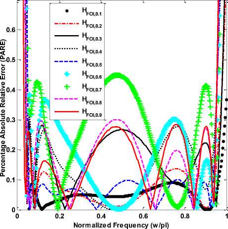
Fig.5. PARE response of RCA designed FOIs

Table 1. Pole- Zero Distribution of Proposed RCA Designed Fractional Order Integrators

RCA designed FOIs	Zeros	Poles
H FOI,0.1 (z-1)	-0.5577, 0.6601, 0.9220, 0.2929, -0.0231	-0.5504, 0.6916, 0.9407, 0.3306, +3.6377e-004
H FOI,0.2 (z-1)	-0.5612, 0.6431, 0.9137, 0.2739, -0.0343	-0.5470, 0.7087, 0.9479, 0.3488, 0.0125
H FOI,0.3 (z-1)	-0.5643, 0.6231, 0.9066, 0.2548, -0.0452	-0.5435, 0.7246, 0.9551, 0.3674, 0.0248
H FOI,0.4 (z-1)	-0.5677, 0.6083, 0.8953, 0.2356, -0.0557	-0.5397, 0.7407, 0.9615, 0.3855, 0.0374
H FOI,0.5 (z-1)	0.2133, 0.5958, 0.8821, -0.5695, -0.0682	-0.5357, 0.4024, 0.7575, 0.9685, 0.0502
H FOI,0.6 (z-1)	0.1965, 0.5714, 0.8757, -0.5744, -0.0753	-0.5311, 0.4223, 0.7698, 0.9775, 0.0629;
H FOI,0.7 (z-1)	0.1765, 0.5534, 0.8643, -0.5777, -0.0842	-0.5283, 0.4398, 0.7893, 0.9785, 0.0759
H FOI,0.8 (z-1)	0.1563, 0.5341, 0.8540, -0.5807, -0.0926	-0.5241, 0.4585, 0.8019, 0.9852, 0.0887
H FOI,0.9 (z-1)	0.1355, -0.1000, 0.5144, 0.8425, -0.5841	-0.5200, 0.4764, 0.8150, 0.9921, 0.1015

-1

1.5

0.5

d о

-0.5

0.1    0.2   0.3    0.4    0.5   0.6    0.7   0.8    0.9     1

Normalized Frequency (w/pi)

Fig.6. Group delay response of RCA designed FOIs

It can be seen from Fig.5 that the proposed integrators; H FOI,0.1 (z^-1) has PARE ≤ 0.08 over 0.04π ≤ ω ≤ 0.97π radians, H FOI,0.2 (z^-1) has PARE ≤ 0.12 over 0.04π ≤ ω ≤ 0.96π radians, H FOI,0.3 (z^-1) has PARE ≤ 0.28 over 0.03π ≤ ω ≤ 0.98π radians, H_FOI,0.4(z^-1) has PARE ≤ 0.27 over 0.04π ≤ ω ≤ 0.96π radians, H_FOI,0.5(z^-1) has PARE ≤ 0.10 over 0.05π ≤ ω ≤ 0.94π radians, H_FOI,0.6(z^-1) has PARE ≤ 0.38 over 0.04π ≤ ω ≤ 0.97π radians, H FOI,0.7 (z^-1) has PARE ≤ 0.42 over 0.04π ≤ ω ≤ 0.97π radians, H FOI,0.8 (z^-1) has PARE ≤ 0.30 over 0.03π ≤ ω ≤ 0.96π radians and H FOI,0.9 (z^-1) has PARE ≤ 0.27 over 0.02π ≤ ω ≤ 0.96π radians. To show efficiency of the proposed FOIs, various existing half order integrators have considered. These half order integrators are Krishna H K,0.5 (z^-1) [14], Gupta-Varshney Visweswaran H GVV,0.5 (z^-1) [15], Gupta-Jain-Jain H GJJ,0.5 (z^-1) [16], and Li-Sheng-Chen H LSC,0.5 (z^-1) [17]. Their transfer functions are given in (40-43).

H GVV,0.5⁽ ? 1 ) =

0.0224(1 - 0.8506 ? ^{- 1})(1 - 0.4708 ? ^{- 1})

(1 + 0.2421 ? ^M0l^:91 + ^

(1 - 0.9631 ? \1 Ш-il¹ ?

(1 - 0.2488 ? ^{- 1})(1 + 0.1311 ? ^{- 1})

D. Comparison of Designed Fractional Order Integrators with the existing FOIs

By observing the frequency response (Fig. 1-6), it can be seen that RCA provides much better approximation than TSE and CFE. The pole-zero distribution of the proposed RCA designed FOIs are shown in Table 1. It can be observed that all of these have poles and zeros inside the unit circle, ensuring their stability.

H GJJ,0.5⁽ ? ^{1 )} =

^HLSC,0.5⁽ ? ^{1 )} =

0.9309-0.9040 ? ^{- 1} - 0.4901 ? ^{- 2}

+ 0.4421 ? "³ + 0.0726 ? "4 -0.0366 ? ^{- 5}

1 - 1.5644 ? ^-1 + 0.0194 ? "² + 0.7243 ? "³

- 0.1174 ? -4 -0.0608 ? ^{- 5}

0.00167-0.006112? ^{- 1} + 0.008409? ^{- 2}

- 0.005208? -3 + 0.00129? -4 -4.785x10 -5 ? ~⁵

1 - 4.488 ? ^- + 8.004 ? ^{- 2} - 7.082 ? -3

+ 3.104 ? - 4 -0.5383 ? ^{- 5}

H K,0.5 ⁽ ? 1 ) =

2338478945881457 ^{- 1}+27482610 ^{- 2}

-4184962т-3-492343?"4+51811 ? 5

2499939 - 6333470 ? -* +55367574 2

• -18716230 ^{- 3} + 161721 ? - 4 -99529? ^{- 5}

  
  

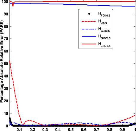
The PARE response and group delay response of the proposed half order integrator (α = 0.5) with above mentioned existing half order integrators over Nyquist frequency range is shown in Fig. 7 and 8, respectively.

Normalized Frequency (w/pi)

Fig.7. PARE response of proposed half order integrator H FOI,0.5 (z^- ) and existing half order integrators; H K,0.5 (z^- ) [14], H GVV,0.5 (z^-1) [15], H_GJJ,0.5(z^- ) [16], H_LSC,0.5(z^-1) [17].

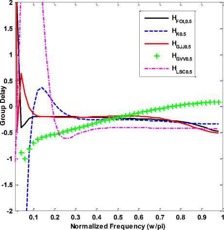
Fig.8. Group delay response of proposed half order integrator H FOI,0.5 (z^- ) and existing half order integrators; H K,0.5 (z^-1) [14], H GVV,0.5 (z^- ) [15], H GJJ,0.5 (z^- ) [16], H LSC,0.5 (z^-1) [17].

It is verified from Fig. 7 that the proposed half order integrator H FOI,0.5 (z^- ) has PARE ≤ 0.10 over 0.05π ≤ ω ≤ 0.94π radians while the existing half order integrator:

Krishna H K,0.5 (z^- ) [14] has PARE ≤ 8.30 over 0.11π ≤ ω ≤ π radians, Gupta-Varshney-Visweswaran H_GVV,0.5(z^- ) [15] has PARE ≤ 96 over 0 ≤ ω ≤ π radians, Gupta-Jain-Jain H GJJ,0.5 (z^- ) [16] has PARE ≤ 2.6 over 0.30π ≤ ω ≤ π radians and Li- Sheng- Chen H_LSC,0.5(z^- ) [17] has PARE ≤ 100 over 0 ≤ ω ≤ π radians.

It is verified from above results (Fig. 5 and 7) that proposed FOIs have very low PARE as compared to the existing ones over the entire Nyquist frequency range. It is also confirmed from Fig. 6 and 8 that the proposed FOIs also have linear phase response as compared to the existing ones.

• V.    Proposed Fractional Order Differentiators and Their Comparison with the Existing Fods

It is observed from Section IV that RCA gives better approximations than TSE and CFE. Here, FODs are obtained by inverting the transfer functions of RCA based FOIs H FOI,α (z^- ) (31-39) in the similar way as used in the design of analog differentiator by Al-Alaoui [26]. Their transfer functions D FOD,α (z^- ) are given in (44-52). The PARE and group delay response of these proposed FODs are shown in Fig. 9 and Fig. 10, respectively.

1.0000-1.4129 ? ^{- 1} + 0.1104 ? -2

D FOD,0.1 ⁽ ? 1 ) = ⁽

+ 0.4400 ? -3 -0.1185 ? -4 + 0.00001 ? -5 -0.9867 + 1.2769 ? -1 + 0.0041 ? -2 -0.4146 ? -3

) (44)

+ 0.0885 ? ^{- 4} + 0.0023 ? ^{- 5}

1.0000-1.4709 ? ^{- 1} + 0.1709 ? ^{- 2}

_D        , -1 _x ,    + 0.4473 ? -3 -0.1338 ? -4 + 0.0016 ? -5

^FOD,0.2           -0.9724+1.2011 ? -1 + 0.0554 ? -2 -0.3964 ? -3

+0.0742 ? ^{- 4} +0.0030 ? ^{- 5}

1.0000-1.5284 ? ^{- 1} +0.2339 ? ^{- 2}

1         + 0.4524 ? -3-0.1495 ? ^{- 4} + 0.0034 ? ^{- 5}

Dpon 0 з( ?  ) = (-------------- i---------?--------7

FOD,⁰.³           -0.956371.1237 ? -1 + 0.1028 ? - 2 -0.3753 ? ^{- 3}

+0.0606 ? ^{- 4} +0.003 5 ? ^{- 5}

1.0000-1.5854 ? ^{- 1} + 0.2995 ? ^{- 2}

1         + 0.4549 ? -3-0.1655 ? ^{- 4} + 0.0054 ? ^{- 5}

Dfod о 4( ?  ) = (--------------------тг fod,0.4\         -0.9448+1.0542? 1 + 0.1453? 2-0.3562? 3

+0.0487 ? ^{- 4} +0.0038 ? ^{- 5}

1.0000-1.6429 ? ^{- 1} + 0.3680 ? ^{- 2}

-1         + 0.4554 ? ^{- 3} -0.1817 ? ^{- 4} + 0.0079 ? ^{- 5}

DFOn0 5⁽ ?  ) = ⁽              i        ?       7

^FOD,0.5           -0.9311+0.9809 ? ^{- 1} + 0.1851 ? ^{- 2} -0.3337 ? ^{- 3}

+0.0362 ? ^{- 4} +0.0041 ? ^{- 5}

1.0000-1.7014 ? ^{- 1} + 0.4412 ? ^{- 2}

-h _ (   + 0.4525 ? -3-0.1986 ? ^{- 4} + 0.0106 ? ^{- 5}

Dfod о б( ?  ) = (------------- j --------т?-------т?

^FOD,0.^6V         -0.9187+0.9131 ? 1 + 0.2204 ? 2 -0.3127 ? ³

+0.0275 ? ^{- 4} +0.0039 ? ^{- 5}

1.0000-1.7552 ? ^{- 1} + 0.5110? ^{- 2}

К ,   + 0.4500 ? -3-0.2158 ? ^{- 4} + 0.0136 ? ^{- 5}    _x (50)

Dfod 0 (??  ) = (--------------- 1----------?--------- t) ^{v 7}

^FOD,0.7            -0.9016 + 0.8405 ? ^{- 1} + 0.2507 ? ^{- 2} -0.2887 ? ^{- 3}

+ 0.0184 ? ^{- 4} + 0.0037 ? ^{- 5}

1.0000-1.8102 : ^{- 1} + 0.5852 : ^{- 2}

D

FOD,0.8

1.5

0.5

2 e

-0.5

-1

( : ^- 1 ) = (

+ 0.4429 : '-0.2 32 5 : ⁴ + 0.0168 : 5 -0.8895+0.7749 z  ■ 0.2784 : "2 -0.2658 : 3

) (51)

+0.0105 : ^{- 4} +0.0034 : ^{- 5}

1.0000-1.8650 : ^{- 1} + 0.6610 : "2

D FOD,0.9^{( :} 1 ) = ⁽

+ 0.4340 : "3 -0.2493 : ⁴ + 0.0203 : 5 -0.8771+0.7089 z ' + 0.3029 : 2 -0.2424 : "³

) (52)

+0.0036 : ^{- 4} +0.0030 : ^{- 5}

0.6

D FOD,0.1

D FOD,0.2

D FOD,0.3

D FOD,0.4

D FOD,0.7

D FOD,0.5

D FOD,0.6

D FOD,0.8

D FOD,0.9

S

0.3

0.2

0.1

0.2

0.4

0.6

0.8

Normalized Frequency (w/pi)

5№

Fig.9. PARE response of proposed FODs

0.5

0.4

D FOD,0.1

D FOD,0.2

D FOD,0.3

D FOD,0.4

D FOD,0.5

D

FOD,0.6

+■ D

FOD,0.7

D FOD,0.8

D FOD,0.9

0.1    0.2    0.3    0.4    0.5    0.6    0.7    0.8    0.9     1

Normalized Frequency (w/pi)

Fig.10. Group delay response of proposed FODs

It can be seen from Fig. 9 that the proposed fractional order differentiators; D FOD,0.1 (z^-1) has PARE ≤ 0.08 over 0.04π ≤ ω ≤ 0.97π radians, D FOD,0.2 (z^-1) has PARE ≤ 0.12 over 0.04π ≤ ω ≤ 0.96π radians, D FOD,0.3 (z^-1) has PARE ≤ 0.28 over 0.03π ≤ ω ≤ 0.98π radians, D_FOD,0.4(z^-1) has

PARE ≤ 0.27 over 0.04π ≤ ω ≤ 0.96π radians, D FOD,0.5 (z^-1) has PARE ≤ 0.10 over 0.05π ≤ ω ≤ 0.94π radians, D FOD,0.6 (z^-1) has PARE ≤ 0.38 over 0.04π ≤ ω ≤ 0.97π radians, D FOD,0.7 (z^-1) has PARE ≤ 0.42 over 0.04π ≤ ω ≤ 0.97π radians, D_FOD,0.8(z^-1) has PARE ≤ 0.30 over 0.03π ≤ ω ≤ 0.96π radians and D_FOD,0.9(z^-1) has PARE ≤ 0.27 over 0.02π ≤ ω ≤ 0.96π radians.

To show the efficiency of the proposed FODs, various existing half order differentiators have been considered. These half order differentiators are Krishna D K,0.5 (z^-1) [14], Leulmi-Ferdi D LFM,0.5 (z^-1), D LFT,0.5 (z^-1) [18]. Their transfer functions are given in (53-55).

D K,0.5^{( :} 1 ) =

2499939-6333470' : ^-1+55367574 ^{- 2}

-1871623a "3+161721 к -4-99529: ~⁵ 2338478^-4588145' : "1+27482610 "2-4184962: "³ -492343: " 4 +51811 : " ⁵

D LFM,0.5 ( ^: 1 ) =

(1.075904»92052;-3.0680788315325 : ^{- 1}+2.8603115S19577 ^{- 2}

-0.7132144891792:^-3-0.2548188S0361843480 : ^{- 5}-0.0999118434380: ')

(1.000000 0 0000002.2610561422849: ^{- 1}+1.3749064744489: ”²

+ 0.1087287045714: ^{- 3}-0.2483486095267:-⁴+8.8262913818929: ^{- 5})

(1.875984в9285498.3586349в4818• : ^{- 1}-0.2390899560122: ^{- 2}

q        , - 1 x _ -0.0796966553374: ^i.053 13 110689 16 : ⁴ 0.0354207:145944: )

^LFT,⁰.⁵           (1.0000000000000-0.2572377881396 ^{- 1}-0.0186107523317: "²

+0.004787388899 1 ^- 3 -0.0014046 7 69357-4+0.0004504 3 12368: ^{- 5})

The PARE response and group delay response of the proposed half order differentiator (α = 0.5) with above mentioned existing half order differentiators over Nyquist frequency range are shown in Fig. 11 and Fig. 12.

It is verified from Fig. 11 that the proposed half order differentiator D FOD,0.5 (z^-1) has PARE ≤ 0.10 over 0.05π ≤ ω ≤ 0.94π radians.

DK0.5

D LFM0.5

D LFT0.5

D FOD,0.5

4.5

3.5

2.5

1.5

0.5

° 2

Qi

0.2

0.4

0.6

0.8

Normalized Frequency (w/pi)

Fig.11. PARE response of proposed half order differentiator D FOD,0.5 (z^-1) and existing half order differentiators; D K,0.5 (z^-1) [14], D LFM,0.5 (z^-1) [18], D LFT,0.5 (z^-1) [18]

D FOD,0.5

D K0.5

D LFM0.5

D LFT0.5

4.5

s 2.5

1.5

2 1

0.5

LU 4

O'

3.5

0.2

0.4

0.6

0.8

Normalized Frequency (w/pi)

Fig.12. Group delay response of proposed half order differentiator D FOD,0.5 (z^-1) and existing half order differentiators; D K,0.5 (z^-1) [14], D LFM,0.5 (z^-1) [18], D LFT,0.5 (z^-1) [18]

The existing half order differentiators: Krishna D K,0.5 (z^-1) [14] has PARE ≤ 7.66 over 0.11π ≤ ω ≤ π radians, Leulmi-Ferdi D_LFM,0.5(z^-1) [18] has PARE ≤ 2.24 over 0.05π ≤ ω ≤ π radians and D_LFT,0.5(z^-1) [18] has PARE ≤ 4.84 over 0.13π ≤ ω ≤ π radians.

It is seen from Figs. 9 and 11 that proposed FODs have very low PARE compared to the existing ones over entire Nyquist frequency range. It is also observed from Figs. 10 and 12 that the proposed FODs have linear phase response compared to the Krishna’s half order differentiator D K,0.5 (z^-1) [14] and Leulmi- Ferdi’s half order differentiator D LFT,0.5 (z^-1) [18].

• VI.    Conclusion

In this paper, design and analysis of digital fractional order differintegrators are discussed. The digital fractional order integrators are designed by direct discretization method using TSE, CFE, and rational Chebyshev approximation. Jain-Gupta-Jain second order integrator is used as a generating function. After that, by modifying these transfer functions fractional order differentiators are designed. The best result is obtained for 0.1 order integrator and differentiator with PARE ≤ 0.08 over the frequency range 0.04π to 0.97π radians/second.

The proposed FODIs have very less PARE over 90% of Nyquist frequency range. Thus, these can be regarded as wideband FODIs. It is also verified that the proposed family of fractional order differintegrators outperforms all the existing FODs and FOIs over the entire Nyquist frequency range. These proposed fractional order differintegrators can be used in variety of practical applications as they have very less PARE and linear phase response over the entire frequency range.