Design of RLS Wiener Smoother and Filter from Randomly Delayed Observations in Linear Discrete-Time Stochastic Systems

Published Online August 2013 in MECS

In the detection and the estimation of the stochastic signal, the estimation problem, given uncertain observations, has been studied extensively. Nahi [1] proposes the recursive least-squares (RLS) estimation procedure for the state vector with the uncertain observations. Here, by the uncertain observation, it means that there is the case where the observed value consists of the observation noise only.

For the observed value with random delays, the estimators for the state vector are also devised [2]-[5]. Matveev and Savkin [6] propose the recursive minimum variance state estimator in linear discrete-time partially observed systems perturbed by white noises for the observed values transmitted with independent delays via communication channels.

The RLS Wiener filter and fixed-point smoother [7] are proposed in linear discrete-time systems. The estimators use the following information. (1) The system matrix. (2) The observation vector. (3) The variance of the state vector in the dynamic model for the signal. (4) The variance of white Gaussian observation noise. By an appropriate choice of the observation vector and state variables, the state-space model, related to the autoregressive moving average (ARMA) model, is introduced. Hence, AR parameters constitute the elements of the system matrix.

In [8], given the uncertain observations, the estimation technique, with the covariance information, is studied. The detection and estimation methods, given the covariance information, are explained [9] in continuous-time stochastic systems.

In [10], the RLS estimation problem of the signal, given the randomly delayed observations, is studied for the additive white noise correlated with the signal. It is assumed that the actual observed value arrives on time or delayed by one sampling time. This is modeled by the delay probability. In the observation equation Bernoulli random variables are used (e.g. see section 2). Recursive one-stage predictor and filter are proposed, based on the innovation approach. Here, both the autocovariance function of the signal and the crosscovariance function of the signal with the observation noise are expressed in the form of the semi-degenerate kernel. Similarly, in [11], the RLS algorithms for the filtering, fixed-point smoothing and fixed-interval smoothing estimates are proposed from delayed observed values, by one sampling time, characterized by the delay probability.

In [12], an RLS Wiener fixed-point smoother and filter are proposed based on randomly delayed observed values by one sampling time in linear discrete-time wide-sense stationary stochastic systems. The observed value y(k) consists of the observed value y(k -1) with the probability p(k) and of y(k) with the probability 1 - p(k). It is assumed that the delayed measurements are characterized by Bernoulli random variables. The observation y(k) is given as the sum of the signal z(k) = Hx(k) and the white observation noise v(k). The RLS Wiener estimators explicitly require the following information: (a) the system matrix for the state vector x(k) ; (b) the observation matrix H; (c) the variance of the state vector x(k); (d) the delayed probability p(k); (e) the variance of white observation noise v(k).

This paper presents an alternative design for the RLS Wiener fixed-point smoother and filter from randomly delayed observed values by one sampling time in linear discrete-time wide-sense stationary stochastic systems. The actual observed value y ( k ) consists of the observed value y ( k -1), at time k -1, with the probability p ( k ), and of y ( k ), at time k , with the probability 1 - p ( k ). It is assumed that the delay measurements are characterized by the Bernoulli random variables (see (1)). y ( k ) is given as the sum of the signal z ( k ) = Hx ( k ) and the white observation noise v ( k ). The proposed RLS Wiener estimators require not only the same information (a)-(d), described in the above regarding [12], but also the following information: (f) the input noise variance concerning the state equation for the augmented vector V ( k ) related with the observation noise. The RLS Wiener estimation algorithms for the fixed-point smoothing estimate and the filtering estimate are proposed. Also, the filtering error variance function of the signal is formulated.

In comparison with the Kalman estimators, the RLS Wiener estimators are advantageous in the point that the RLS Wiener estimators do not use the information of the input noise variance and the input matrix in the state equation for the signal. The less information in the estimators might avoid the degradation of the estimation accuracy caused by the inaccurate information on the state-space model. In [7], the RLS Wiener filter and fixed-point smoother are proposed in linear discretetime stochastic systems. The estimators need the information of the system matrix, the observation vector, the variance of the state vector and the variance of white observation noise. In addition, in linear discretetime stochastic systems, the following RLS Wiener estimators are studied, i.e. the Chandrasekhar-type RLS Wiener fixed-point smoother, filter and predictor [13], the square-root RLS Wiener fixed-point smoother and filter [14] and the RLS Wiener FIR filter [15], etc.

The organization of this paper is as follows. In section 2, the least-squares fixed-point smoothing problem, from the randomly delayed observations, is formulated. Theorem 1, in Section 3, presents the RLS Wiener fixed-point smoothing and filtering algorithms. A numerical simulation example, in section 4, shows the estimation characteristics of the current filter and the fixed-point smoother with the randomly delayed observed values by one sampling time.

II. Least-Squares Fixed-Point Smoothing Problem

Let an m-dimensional observation equation be given by

y ^{( k} ) = ⁽¹ - Y (^k))y ^{( k} ) + Y ^{( k} ) y ^{( k} - 1), y ( k ) = z ( k ) + v ( k ), z ( k ) = Hx ( k )

in linear discrete-time stochastic systems. It is assumed that the observation at each time k >  1 can either be delayed by one sampling period, with a known probability p ( k ), or updated, with a probability 1 - p ( k ). { y ( k ); k >  1} denotes a sequence of independent Bernoulli random variables (a binary switching sequence taking the values 0 or 1 with P [Y( k ) = 1] = p ( k ) . In applications of communication networks, { y ( k ); k >  1} is usually taken to represent the random delay from sensor to controller, and the assumption of a one-step sensor delay is based on the reasonable supposition that the induced data latency from the sensor to the controller is restricted so that it may not exceed the sampling period [4]. Here, z ( k ) is a signal vector, H is an m x n observation matrix, x ( k ) is a zero-mean state vector and v ( k ) is a zero-mean white observation noise. It is assumed that the signal, the Bernoulli variables sequence and the observation noise are mutually independent.

Let the auto-covariance function of v ( k ) be given by

E [ v ( k ) v ^T ( s )] = R ( k ) 5 _K ( k - s ), R ( k ) >  0

Here, 5 (.) denotes the Kronecker 5 function. By denoting

Y ^{( k} ) = [ / ^{( k} ) I m x m   ⁽¹ — Y ^(k )) I m x m ] ,

z ( k ) =

Z ( k - 1) z ( k )

V ( k ) = Y ( k )V ( k ),

V ( k ) =

v ( k - 1) v ( k )

from (1), we obtain

y ( k ) = Y ( k ) z ( k ) + v ( k ) .               (4)

By denoting

H =

H

H

x ( k ) =

x ( k - 1) x ( k )

from (1) and (3), the observation equation (4) is also written as

y ( k ) = y ( k ) Hx ( k ) + v (k ) ,                 (6)

K x ^{( s} , ^s ) =

since

z ^{( k} ) =

z ( k - 1) z ( k )

Hx ( k - 1) Hx ( k )

= Hx ( k ).

Let K_x ( k , s ) = K ( k - s ) represent the auto-covariance function of the state vector x ( k ) in wide-sense stationary stochastic systems [16], and let K ( k , s ) be expressed in the form of

Kx(k,s)

Г A ( k ) B T ( s ), I B ( s ) A T ( k ),

0 < s < k,0 < k < s,

A ( k ) = Ф ^k , B T ( s ) = Ф^- s K ( s , s ).

Here, Ф is the transition matrix of _x ( k ).

Let the state-space model for x ( k ) be described as

x ( k + 1) = Ф x ( k ) + Gw k ),

E [ w ( k ) w ^T ( s )] = Q ( k ) ^ k ( k - s ),

where B is an n x l input matrix and _w ( k ) is white i n put noise with the auto-covariance function of (9). Let Ф represent the system matrix for x ( k ). From

x ( k )

x ( k + 1)

Ф is given by

Ф =

+

0   I n x n

0 Ф

0  In x n   x (k -1)

0 Ф ][ x ( k )

0 Gw ( k )

Let K ( k , s ) represent the auto-covariance function

of x ( k ) . K ( k , s ) is expressed in the form of

K_x ( t , s )

Г A ( k ) B ^T ( s ),

B ( s ) A ^T ( t ),

0 < s < k,0 < k < s,

A ( k ) = Ф ^k , B ^T ( s ) = Ф^{- s} K x ( s , s ).

Here, K ( s , s ) = K_ (0) is expressed as

K x (0)    K x (0) Ф T

Ф K x (0)    K x (0)

In (11), Ф is a singular matrix. However, in the estimation algorithm of Theorem 1, the inverse matrix of Ф is not included.

Let K (.,.) denote the auto-covariance function of V ( k ). From (2) and (3), K_v ( k , k ) and K_v ( k +1, k ) are given by

K v ( k , k ) = E \_ V ( k )V ^T ( k ) ]

= E

v ( k - 1) v ( k )

[ v ^T ( k - 1)   v T ( k ) ]

R ( k - 1)    0

0      R ( k )

K ( k + 1, k ) = E [ V ( k + 1)V ^T ( k ) ]

= E

v ( k )

v ( k + 1)

0   R ( k )

[ v ^T ( k - 1)   v ^T ( k ) ]

From (14) and K_v ( k + i , k ) = 0, i > 2, the auto-

covariance K ( k , s ) is given by

A v ( k ) B V (s ),  0 <  s <  k ,

B v ( s ) A T ^T ( t ),   0 <  k <  s ,

A v ( k ) = Ф V ,   B ^T ( s ) = Ф V K y ( s , s ),      (15)

Ф V

m x m

Let the state equation for V ( k ) be given by

V ( k + 1) = Ф_Г V ( k ) + U ( k ),

E [ U ( k)U ^T ( s )] = R u ( k ) 5 k ( k - s ),

in terms of white input noise U ( k ) with the variance R . It is found that for the expressions

K_y ( k +1, k +1) = E [ V ( k + 1) V ^T ( k +1)],

K_v ( k, k ) = E[V ( k)V^T ( k )], in the wide-sense stationary stochastic systems, the following relationships hold.

Ru ( k ) = K_v ( k + 1, k + 1)

-ф л ( k , k ) ф T , K_v ( k + 1, k + 1) = K_v ( k , k )

= K v (0).

Let the fixed-point smoothing estimate x ˆ ( k , L ) of x ( k ) at the fixed point k be expressed by

L x (k, L) = £ h (k, i, L) y (i)                 (18)

i = 1

in terms of the observed values { y ( i ),  1 <  i <  L } . In (16),

h ( k , i , L ) is a time-varying impulse response function.

Let us consider the estimation problem, which minimizes the mean-square value (MSV)

J = E [|| x ( k ) - x ( k , L )|| 2 ]                    (19)

of the fixed-point smoothing error. From an orthogonal projection lemma [16],

L

x ( k ) — £ h ( k , i , L ) y ( i ) X y ( s ), i = 1

1 < s < L, the impulse response function satisfies the Wiener-Hopf equation

E [ x ( k ) y T ( s )] =

5> ( k , i , L ) E [ y ( i ) y^T ( s )].

i = 1

Here ‘ X ’ denotes the notation of the orthogonality.

By setting p ( k ) = [ p ( k ) I m x m  (1 - p ( k )) I m x m ] , from ⁽⁴⁾

and (6), the left hand side of (21) is rewritten as

E [ x ( k ) y^T ( s )]

= E [ x ( k )( Y ( s ) z ( s ) + v ( s )) ^T ]

= E [ x ( k ) z^T ( s ) y ^t ( s )]

= E [ x ( k ) x^T ( s )] H^T

^[ P ^{( s} ) I m x m  ⁽¹ — P ^{( s} )) I m x m Г

= K x ( k , s ) H^Tp^T ( s ).

E [ y ( i ) y^T ( s )]

= E [( Y ( i ) H ( i )

+ v ( i ))( Y ( s ) Hx ( s )

+ v ( s )) ^T ]

= E y [ y ( i )( HK x ( i , s ) H^T + K v ( i , s )) Y ^T ( s )].

Here, e^ [.] denotes the notation of expectation with respect to y(-) . Substituting (22) and (23) into (21), we obtain

K x ( k , s ) H^T p ^T ( s )

= ^Th ( k , i , L ) E y [ y ( i )( HK x ( i , s ) H^T       (24)

i = 1

+ K v ( i , s )) Y T ( s )].

In terms of the introduced quantities, K vu ( i , s ) = E [ V ( i)U^T ( s )], K uv ( i , s ) = E [ U ( i)V^T ( s )], it is shown that

K v ( i , s ) = E [ V ( i )V^T ( s )]

= E [( Ф v V ( i - 1)

+ U ( i - 1))( Ф v V ( i - 1) + U ( i — 1)) ^T ]

= ф v K v ( i , s ) Ф V                           (25)

+ Ф v K vu ( i , s )

+ K uv ( i , s ) Ф T + R u ( i ) S k ( i - s ).

Substitution of (25) into (24) yields

K x ( k , s ) H^T p ^T ( s )

= £ h ( k, i, L ) Ey [Y (i)( HK( i, s ) HT i=1

+ Ф t K t ( i , s ) Ф Т                          (26)

+ Ф t K tu ( i , s )

+ K ut ( i , s ) Ф T

+ R u ( i )5_K ( i - s )) Y ^T ( s )].

Namely,

Also, from (3) and (6), E[y(i)yT(s)] is rewritten as h ( k, 5, L) Ey [y (s ) Ru ( s )YT (s)]

= K x ( k , s ) H T P T ( s )

• - T h ( k , i , L ) E y [ y ( i )( HK x ( i , s ) H T i = 1                                                             ⁽2 ⁷⁾

+ Ф v K v ( i , s ) Ф V

+ Ф v K vu ( i , s )

+ K uv ( i , s ) Ф V ) y ^t ( s )].

and since

E [Y (k)] = P (k),

K uv ( s , s ) = E [ U ( s )V^T (s )] = 0,             (28)

K vu ( s , s ) = E [ V ( s ) U^T ( s )] = 0,

• (27) is written as

h ( k , s , L )( E y [ Y ( s ) R u ( s ) Y ^T ( s )]

+ Ey [Y (s )(HK( s, s ) HT

^{+ Ф} V K V ^{( s} , ^{s ) Ф} V ^{) Y} T ^{( s )]}

• -    P ( s )( HK( s , s ) H^T

^{+ Ф} V K V ^{( s} , ^{s ) Ф} V ) ^{pT ( s} ))

= K x ( k , s ) H T P T ( s )                        ⁽²⁹⁾

• - £ h ( k , i , L ) p ( i )( HK x ( i , s ) H^T

+ Ф v K v ( i , s ) Ф T

+ Ф K vu ( i , s )

^{+ K}uv ⁽ i , ^{s ) Ф} V ) ^p T ^{( s} )

Consequently, the optimal impulse response function h ( k , s , L ) satisfies

h ( k , s , L ) R ( s )

= K ^ ( k , s ) H T P T ( s )

• - f> ( k , i , L ) P ( i )( HK ( i , s ) H^T 7=7                                             (30)

+ Ф v K v ( i , s ) Ф T

+ Ф v K vu ( i , s )

+ Kuv (i, s)ФV )PT (s), where

R ( s )

= E y [ Y ( s ) R u ( s ) Y T ( s )]

+ Ey [y (s)(HKx (s, s) HT

+ Ф v K v ( s , s ) Ф V ) Y ^T ( s )]

• - p ( s )( HK( s , s ) H^T

+ Ф v K v ( s , s ) Ф V ) P^T ( s ).

• III. RLS Wiener Estimation Algorithms

Under the linear least-squares estimation problem of the signal z ( k ) in section 2, Theorem 1 shows the RLS Wiener fixed-point smoothing and filtering algorithms, which use the covariance information of the signal and observation noise.

• Theorem 1

Let the auto-covariance function K ( k , s ) of the state vector x ( k ) be expressed by (8), let the variance of white observation noise v ( k ) be R ( k ) and let the variance of U ( k ) in the state equation (16) for у ( k +1) be R ( k ) . Then, the RLS Wiener algorithms for the fixed-point smoothing at the fixed point k and the filtering estimate of the signal z ( k ) consist of (32)-(54) in linear discrete-time stochastic systems with randomly delayed observed values by one sampling time.

Fixed-point smoothing estimate of the signal z ( k ) :

z( k , L ) = Hx ( k , L )

.x ( k , L ) = [ 0   I ] ; X ( k , L ),                       (32)

.x ( k , L ) = [ 0   I ] jX ( k , L )

Fixed-point smoothing estimate of x ( k ) : x ^ˆ ( k , L )

x ( k , L ) = jX ( k , L - 1) + h ( k , L , L )( y ( L ) - P ( L )( H Ф X ( L - 1, L - 1) + Ф V V₂(L - 1, L - 1) + Ф v V₃ -1,L -1))),

	" H	0"
H =
	_ 0	H	,
	■ H	0"	■ 0 I"
H =			, Ф^ =
	0	H	V   0  0

h ( k , L , L ) = [ K x ( k , k )( Ф T ) L - k H T p T ( L )					q з ( k , L ) = q з ( k , L - 1) Ф T
- q^k , L - 1) Ф T H T p T ( L )					+ h ( k , L , L ) p ( L )( R u ( L )
- q 2 ( k , L - 1)( Ф T )2pT ( L )					- ( H Ф S 13 ( L - 1) Ф T				(37)
- q з ( k , L - 1) Ф V p T ( L )] x [ R ( L )					+ ( Ф v ) 2 S 23 ( L - 1) Ф T
	+ p ( L )( HK x ( L , L )				+ Ф v S 33	( L - 1) Ф T )),
	- ( H Ф S ^L - 1) Ф T + ( Ф v ) 2 S 21 ( L - 1) Ф T				q 3 ( k , k ) =	S 13 ( k )
	+ Ф v S 31 ( L - 1) Ф T )) HTpT ( L )				Filtering	estimate   of	the   signal		z ( L )    :
	+ p ( L )( Ф v K v ( L , L )				Z( L , L ) = Hx ( L , L )
	- ( H Ф S 12 ( L - 1) Ф T				x( L , L ) =	0 I ] x ( L , L ),
	+ ( Ф v ) 2 S 22( L - 1) Ф v + Ф v S 32 ( L - 1) Ф T )) Ф T pT ( L )				x ( L , L ) =	"x(L - 1, L - 1)" _    x( L , L )    _			(38)
	+ p ( L )( R u ( L )
	- ( H Ф S 1з ( L - 1) Ф v				Filtering estimate of x ( L ): x ˆ ( L , L )
	+ ( Ф v ) 2 S 2з ( L - 1) O T			(34)	.x ( L , L ) =	Ф x ( L - 1, L - 1)
	+ Ф vS 33	( L - 1) O T )) pT ( L )] - 1 ,			+ G 1 ( L )( y ( L )
						- p ( L )( H Ф x ( L	- 1, L -	1)
K x ( L , L ) =	" K (0)	K (0) Ф T"				ˆ			(39)
	xx Ф K x (0)    K x (0) _		,		+ ( Ф v )2 v 2 ( L - 1, L - 1)
	" R  0 "				+ Ф v v 3 ( L - 1, L		- 1))),
K v ( L , L ) =	0 r				x (0,0) = 0
q i ( k , L ) = q i ( k , L - 1) Ф T					Filtering estimate of  ( L ) :
+ h ( k , L , L ) p ( L )( HK- ( L , L )					Ф v v 2 ( L -	1, L - 1) + v 3( L	- 1, L -	1))
- ( H Ф S ,( L - 1) Ф		T		(35)
+ (Фv )2 V 21 ( L - 1) Ф T					2( L , L )	= Ф v v 2( L - 1, L	- 1)
+ Ф v S 31 ( L - 1) Ф T )),					+ G 2 ( L )( y ( L )
q 1 ( k , k ) = S n( k )						- p ( L )( H Ф x ( L - 1, L		- 1)	(40)
					+ ( Ф v )	2 v 2 ( L - 1, L - 1)
q 2 ( k , L ) =	q 2 ( k , L	- 1) Ф T			-
+ h ( k , L , L ) p ( L )( Ф v K v ( L , L )					+ Ф v v 3	( L - 1, L - 1))),
- ( H Ф S .,( L - 1) Ф T				(36)	v 2 (0,0) =	0
+ ( Ф, )2 S, ,( L - 1) Ф ',							1) --- /X
+ Ф v S 32	( L - 1) Ф T )),				v , ( L , L ) =	Ф v v 3 ( L - 1, L -
q 2 ( k , k ) =	S 12 ( k )				+ G 3 ( L )( y ( L ) - p ( L )( H Ф x ( L -			1, L	- 1)
					+ ( Ф v )2 v 2 ( L - 1, L - 1)				(41)
					+ Ф v K3( L - 1, L - 1))),
					v 3 (0,0) =	0

Design of RLS Wiener Smoother and Filter from Randomly Delayed Observations in Linear Discrete-Time Stochastic Systems			7
Filtering variance function of x ˆ ( L , L ) : 5 n( L ) = E[ X ( L , L ) X T ( L , L )]		5 22 ( L ) = Ф v 5 22 ( L - 1) Ф V + G 2 ( L ) p ( L )( Ф v K v ( L , L )
5 n( L ) = Ф 5 u( L - 1) Ф T + G i ( L ) p ( L )( HK x ( L , L ) - ( H Ф 5 Д L - 1) Ф T	(42)	- ( H Ф 5 12 ( L - 1) Ф V + ( Ф V )2 5 22 ( L - 1) Ф V + Ф v 5 32 ( L - 1) Ф V )),	(46)
+ ( Ф V )2 5 21 ( L - 1) Ф T		5 22 (0) = 0
+ Ф v S 31 ( L - 1) Ф T )), 5 11 (0) = 0		Cross-variance function of V ˆ ( L , L ) with V ˆ ( L , L ) 5 2з ( L ) = E [ jV 2( L , L )V> 3T ( L , L )]
Cross-variance function of x ˆ ( L , L ) with S 12( L ) = E [ X ( L , L )V ( L , L )] 5 12( L ) = Ф 5 12 ( L - 1) Ф T + G 1 ( L ) p ( L )( Ф v K v ( L , L )	V ˆ 2 ( L , L ) :	5 23 ( L ) = Ф v 5 23 ( L - 1) Ф T + G 2 ( L ) p ( L )( R u ( L ) - ( H Ф 5 13 ( L - 1) Ф T + ( Ф v ) 2 5 23 ( L - 1) Ф T	(47)
- ( H Ф 5 12 ( L - 1) Ф V + ( Ф v )2 5 22 ( L - 1) Ф T + Ф v 5 32 ( L - 1) Ф V )), 5 12 (0) = 0	(43)	+ Ф v 5 33 ( L - 1) Ф Т )), 5 23 (0) = 0 5 31 ( L ) = Ф v 5 31 ( L - 1) Ф T + G 3 ( L ) p ( L )( HK( L , L )
Cross-variance function of x ˆ ( L , L ) with	V ˆ 3 ( L , L ):	- ( h Ф s x l - 1) Ф T
5 B( L ) = E [ X ( L , L VT ( L , L )] 5 13( L ) = Ф 5 13( L - 1) Ф V + G 1 ( L ) p ( L )( R u ( L ) - ( H Ф 5 13( L - 1) Ф T	(44)	+ ( Ф V ) 2 5 21 ( L - 1) Ф T + Ф v 5 31 ( L - 1) Ф T )), 5 31 (0) = 0, 5 31 ( L ) = 5 T 3 ( L ) 5 32 ( L ) = Ф v 5 32 ( L - 1) Ф V	(48)
+ ( Ф v )2 5 2з ( L - 1) Ф T		+ G 3 ( L ) p ( L )( Ф v K v ( L , L )
+ Ф v 5 зз ( L - 1) Ф T )), 5 13 (0) = 0 5 21 ( L ) = Ф v 5 21 ( L - 1) Ф T + G 2 ( L ) p ( L )( HK x ( L , L ) - ( H Ф 5 / l - 1) Ф T + ( Ф V ) 2 5 21 ( L - 1) Ф T + Ф v 5 31 ( L - 1) Ф T )),	(45)	- ( H Ф 5 12( L - 1) Ф T + ( Ф t ) 2 5 22 ( L - 1) Ф T + Ф t 5 32 ( L - 1) Ф T )), 5 32 (0) = 0,   5 32 ( L ) = 5 2 T 3 ( L ) Filtering variance function of V ˆ ( L , L ) : S ( L ) 5 33 ( L ) = Ф t 5 33 ( L - 1) Ф T + G 3 ( L ) p ( L )( R u ( L )	(49)
5 21 (0) = 0,   5 21 ( L ) = 5 1 T 2 ( L )		- ( H Ф 5 13 ( L - 1) Ф Т + ( Ф T )2 5 23 ( L - 1) Ф T	(50)
Filtering variance function of V ( L , L ) : S ( L )		+ Ф t 5 33 ( L - 1) Ф T )), 5 33 (0) = 0

Filter gain for x ˆ ( L , L ): G ( L )

G i ( L ) = [ K x ( L , L ) H T p T ( L )

• - Ф S X L - 1) Ф T H T p T ( L )

• - Ф S ^( L - 1)( Ф V )² p^T ( L )

• - Ф S 13 ( L - 1) Ф V p T ( L )]

x [ R ( L ) + p ( L )( HK x ( L , L )

• -    ( H Ф S X L - 1) Ф ^T

+ ( Ф V )² S 21 ( L - 1) Ф ^T

+ Ф V S 31 ( L - 1) Ф ^T )) H T p T ( L )

• +    p ( L )( Ф V K V ( L , L )

• -    ( H Ф S 12 ( L - 1) Ф V

+ ( Ф V )² S 22 ( L - 1) Ф V

+ Ф V S 32 ( L - 1) Ф V )) Ф V p T ( L )

+ p ( L )( R u ( L )

• - ( H Ф S 13 ( L - 1) Ф V

+ ( Ф V )² S 2з ( L - 1) Ф V             (51)

+ Ф V S зз ( L - 1) Ф V )) p^T ( L )]" 1

Filter gain for V ^ˆ ( L , L ): G ( L )

G 2 ( L ) = [ K v ( L , L ) Ф V p^T ( L )

-Ф v S ₂ 1 ( L - 1) Ф ^TH^Tp^T ( L )

• - Ф v S 22 ( L - 1)( Ф V )² p^T ( L )

• - Ф v S 2з ( L - 1) Ф V p T ( L )]

x [ R ( L ) + p ( L )( HK x ( L , L )

• -    ( H Ф S^L - 1) Ф ^T

+ ( Ф V )² S 21 ( L - 1) Ф ^T

+ Ф v S 31 ( L - 1) Ф ^T )) H^Tp^T ( LL)

• +    p ( L )( Ф V K V ( L , L )

• -    ( H Ф S ^C L - 1) Ф V

+ ( Ф v )² S 22 ( L - 1) Ф V

+ Ф v S 32 ( L - 1) Ф V )) Ф V p^T ( L )

+ p ( L )( R u ( L )

• - ( H Ф S 13 ( L - 1) Ф V

+ ( Ф v )² S 2з ( L - 1) Ф V             (52)

+ Ф v S зз ( L - 1) Ф V )) p^T ( L )]" 1

Filter gain for V ( L , L ) : G ( L )

G 3 ( L ) = [ R u ( L ) p^T ( L )

-Ф v S 31 ( L - 1) Ф T H^Tp^T ( L )

• - Ф v S 32 ( L - 1)( Ф V )² p^T ( L )

• - Ф v S зз ( L - 1) Ф V p T ( L )]

x [ R ( L ) + p ( L )( HK x ( L , L )

• -    ( H Ф S ,( L - 1) Ф ^T

+ ( Ф V )² S 21 ( L - 1) Ф ^T

• +    Ф v S 31 ( L - 1) Ф ^T )) H^Tp^T ( L )

+ p ( L )( Ф v K v ( L , L )

• - ( H Ф S 12 ( L - 1) Ф V

+ ( Ф v )² S 22 ( L - 1) Ф V

+ Ф v S 32 ( L - 1) Ф V )) Ф V p^T ( LL)

+ p ( L )( R u ( L )

• -    ( H Ф S 13 ( L - 1) Ф V

• +    ( Ф v )² S 2з ( L - 1) Ф V             (53)

+Ф v S зз ( L - 1) Ф V )) p^T ( L )] " *

R ( L ) = E _y [ Y ( L ) R u ( L ) y ^T ( L )]

+ E y [ Y ( L )( HK( L , L ) H T

+ Ф v K v ( L , L ) Ф V ) Y ^T ( L )]

• -    p ( L )( HK x ( L , L ) H^T           (54)

+ Ф vKv (L, L )Ф V ) pT (L ), p (L ) = E [Y (L)]

= [ p ( L ) I m x m  (1 - p ( L )) I m x m

Y ( L ) = [ Y ( L ) I , x m  (1 - Y ( L )) I .......]

Proof of Theorem 1 is deferred to the Appendix.

From [Theorem 1], it is found that the filtering error variance function P ^~ ( L ) of the signal z ( L ) is given by

P z ( L ) = K z ( L , L )

• -    HH 1 S 11 ( L )) H T H^T ,             (55)

H1 =[ 0 n x n   In x n ] , where K (L, L) represents the covariance function of z(L).

IV. A Numerical Simulation Example

Let a scalar observation equation be given by y (k) = (1 - r( к )) y ( к)

+ / ⁽ к ) y ⁽ к ^- 1),

E_y Y ( к )] = P (к ),

_^Y                                              (56)

y ( к) = z (к) + v (к ), z (к) = Hx ( к),

E [ v(к ) v(s )] = R5_K (к - s ).

Let the observation noise v ( k ) be zero-mean white Gaussian process with the variance R , N (0, R ). (56) is also written as

У ^{( к} ) = У ^{( к} ) z ^{( к} ) ⁺ v ^{( к} ),

У ^{( к} ) = [ / ^{( к})  ⁽¹ - У ⁽.^к )) ] ,

v ( к ) = у ( к ) [ v ( к - 1)   v(к ) ] ^Г ,                (57)

Hence, H and x ( k ) are given by

H =	H (	I 0' H _ x, ( к	= 1)		1 0	0  0  0" 0  1 0 "x 1 ( к - 1)"	(60) .
x ( k )	— =	x 2( к - 1) x 1 ( к )			— =	x 1( к ) x i ( к )
		x 2 ( к )		-		_ x 1 ( к + 1) _

From x ( k ) , the signal z ( k ) is calculated by

z ( к ) = [ 0  0  1  0 ] x ( к )

= [ 010 0 ] x ( к ) = x ( к ).

The auto-covariance function of the signal z ( k ) is given by [8]

z ^{( к} ) =

z ( к - 1) z ( k )

Hx ( к - 1) Hx ( k )

= Hx ( к ).

Let the signal z ( k ) be generated by the second-order AR model.

K (0) = ст 2 ,

K ( m ) = ст ² {-- “^ -^--

[( a - a )( aa + 1)] a ( a ² - 1)^ 2    )

--} [( a - a )( aa + 1)]

0 <  m ,

a, a = (-ai ± 4a 12 - 4a2) / 2.

z ( к + 1) = - az ( к )

- a₂z ( к - 1) + w ( к ),

E [ w ( к ) w ( s )] = ст²^ ( к - s ),

a =- 0.1,   a ₂ =- 0.8, ст = 0.5.

The state-space model for z ( k ) is given by

From

K x ( к , к ) =	" K (0) _ K (1)	K (1)" K (0) _
■ 0	1 "
ф =	,
_ - a 2	- a 1 J

z ( к ) = Hx ( к ) = x ( к ),

H = [1

0 ] , x ( к ) =

x ( к + 1) x ₂ ( к + 1)

x ₁( k ) x ( k )

0     1     x 1 ( к )

- a₂   - a,   x ₂ ( к )

+

w ( k ).

Ф and K (0) are given by

				"0	0	1	0 "
	"0	I"		0	0	0	1
ф =	0	ф	=	0	0	0	1
				_ 0	0	— a^	- a 1 J

K x (0) =

K x (0)   K x (0) Ф ^T

. Ф K x (0)    K x (0)

	"       K (0)	K (1)	K (1)	- a 2 • K (0) - ax	• K (1)"
	K (1)	K (0)	K (0)	- a 2 • K (1) - a1	K (0)
	K (1)	K (0)	K (0)	K (1)
	_- a 2 • K (0) - ax • K (1)	- a 2 • K (1) - a • K (0)	K (1)	K (0)

K (0) = 0.25, K (1) = 0.125.

From     (54),      (65),      H      in     (60),

P(L) = E [/(L) 1 - Y(L)] = [p(L)  1 - P(L)J   R(L) is calculated as

R ( L ) = E _y [ y ( L ) R u ( L ) y ^T ( L )]

+ E _y [ y ( L )( HK x ( L , L ) H^T

+ Ф V K V ( L , L ) Ф y ( L )]

- p ( L )( HK x ( L , L ) H^T

+ Ф V K V ( L , L ) Ф T ) p^T ( L )

= R u ( L ) + p ( L )( R + 2( K (0) - K (1))

- p ²( L )( R + 2( K (0) - K (1)), R u ( L ) = K v ( L + 1, L + 1)

-Ф V K V ( L , L ) Ф V =

0 R

Ф V =

K v ( L , L ) = K v ( L + 1, L + 1) =

R

0 R

by taking into account E [ y ( L ) ] = E [ y ² ( L )] = p ( L ).

Substituting H , Ф, K x ( L , L ) = K x (0), p ( L ) = [ p ( L ) 1- p ( L )], R_n ( L ) and R ( L ) into the RLS Wiener estimation algorithms in Theorem 1, the filtering and fixed-point smoothing estimates are calculated recursively.

Fig.1 illustrates the fixed-point smoothing estimate z(k , k + 5) vs. k for the probability p ( k ) = 0.1 and the white Gaussian observation noise N (0,0.3²). The probability p ( k )that the observed value y ( k -1) arrives, with one sampling time delay, at time k is 0.1 . The probability 1 - p ( k ) that the observed value y ( k ) arrives at time k is 0.9 . Fig. 2 illustrates the mean-square values (MSVs) of the filtering errors z ( k ) - ^:z(k , k )and the fixed-point smoothing errors z ( k ) - ,z( k , k + Lag ), Lag = 2, vs. the probability p ( k ) for the white Gaussian observation noise N (0,0.3²) . The probability p ( k ) = 0 corresponds to the case where only the observed value y ( k ) is used in calculating the filtering estimate z ˆ( k , k ) and the fixed-point smoothing estimate z( k , k +1).

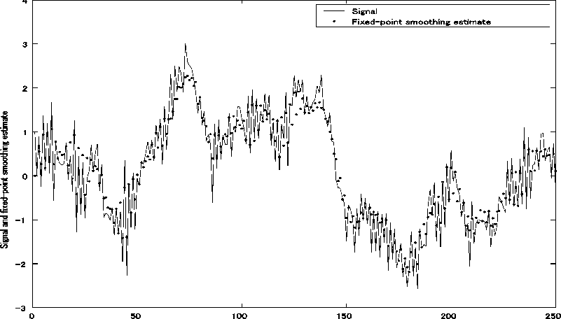
Fig. 1: ixed-point smoothing estimate Z ( k , k + 5) vs. k for the probability p ( k ) = 0.1 and the white Gaussian observation noise N (0,0.3²).

In Fig. 2, both for the filter and the fixed-point smoother, the MSVs tend to increase as the probability p(k\ 0 < p(k) < 0.5, increases. Moreover, the rate of decrease of the MSV of the fixed-point smoothing errors, in comparison with that of the filter, is significant for 0.5 < p(k) < 1.0. From Fig. 2, in the fixed-point smoother, the estimation accuracy is considerably improved for 0.5 < p (k) < 1.0 in comparison with the filter.

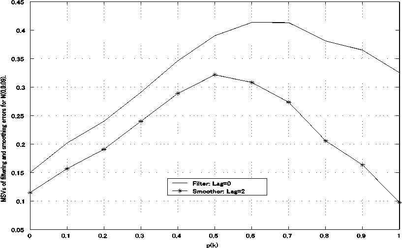
Fig. 2: Vs of the filtering errors z ( k ) - z ( k , k )and the fixed-point smoothing errors _z ( k ) — z ( k , k + Lag ), Lag = 2, vs. the probability p ( k ) for the white Gaussian observation noise N (0 0 3²)

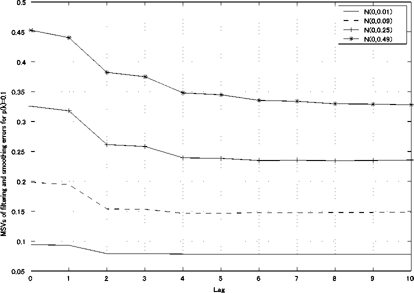
Fig. 3: SVs of the filtering errors z ( k ) — z ( k , k ) and the fixed-point smoothing errors z ( k ) — Z ( k , k + Lag ) vs. Lag , 0 <  Lag <  10, for the white Gaussian observation noises N (0,0.1²), N (0,0.3²), N (0,0.5²) and N (0,0.7²) under the probability p ( k ) = 0.1.

Fig. 3 illustrates the MSVs of the filtering errors z ( k ) - z ( k, k ) and the fixed-point smoothing errors z ( k ) - z(k , k + Lag ) vs. Lag , 0 <  Lag < 10, for the white Gaussian observation noises N (0,0.1²) , N (0,0.3²) , N (0,0.5 2 ) and N (0,0.7 2 ). For Lag = 0, the MSV of the filtering errors z ( k ) - z ( k , k ) is shown. As Lag increases, the MSVs gradually decrease. Hence, the estimation accuracy of the fixed-point smoother is superior to that of the filter. For the white Gaussian observation noise with larger variance, the MSVs of the filtering errors and the fixed-point smoothing errors increase and the estimation accuracy is degraded. Here, the MSVs of the fixed-point smoothing and filtering errors           are           evaluated           by

2000 Lag

£ £ ( z ( k ) - z ( k , k + j )) 2 /(2000 X Lag ) and k = 1 j = 1

£ ( z ( k ) - z( k , k )) 2 /2000. .

k = 1

• V. Conclusions

In this paper, the alternative RLS Wiener fixed-point smoother and filter are designed from observations randomly delayed by one sampling time in linear discrete-time stochastic systems. The probability of the arrival of the observed value y ( k ) at time k is 1 - p ( k ) and the probability of the arrival of the observed value y ( k -1) at time k is p ( k ). In comparison with the estimators in [12], the information of the input noise variance of the state equation for the augmented vector V ( k ), related with the observation noise, is used additionally.

A numerical simulation example shows that the proposed estimation technique with the randomly delayed observed values is feasible. From Fig. 2 and Fig. 3, in the fixed-point smoother, the estimation accuracy is considerably improved for 0.5 <  p ( k ) < 1.0 in comparison with the filter. As Lag increases, the MSV of the fixed-point smoothing errors gradually decreases. Hence, the estimation accuracy of the fixed-point smoother is superior to that of the filter.

The RLS Wiener estimators do not use the information from the variance Q ( k ) of the input noise w ( k ) and the input matrix G in the state equation (9), in comparison with the estimation technique [2]-[5]. Hence, in the RLS Wiener estimation technique, it is not necessary to take account of the degraded estimation accuracy caused by the modeling errors for Q ( k ) and G .