Design Parallel Linear PD Compensation by Fuzzy Sliding Compensator for Continuum Robot

Published Online November 2013 in MECS DOI: 10.5815/ijitcs.2013.12.12

Continuum robots represent a class of robots that have a biologically inspired form characterized by flexible backbones and high degrees-of-freedom structures [1]. The idea of creating “trunk and tentacle” robots, (in recent years termed continuum robots [1]), is not new [2]. Inspired by the bodies of animals such as snakes [3], the arms of octopi [4], and the trunks of elephants [5], [6], researchers have been building prototypes for many years. A key motivation in this research has been to reproduce in robots some of the special qualities of the biological counterparts. This includes the ability to “slither” into tight and congested spaces and (of particular interest in this work) the ability to grasp and manipulate a wide range of objects, via the use of “whole arm manipulation” i.e. wrapping their bodies around objects, conforming to their shape profiles. Hence, these robots have potential applications in whole arm grasping and manipulation in unstructured environments such as rescue operations. Theoretically, the compliant nature of a continuum robot provides infinite degrees of freedom to these devices. However, there is a limitation set by the practical inability to incorporate infinite actuators in the device. Most of these robots are consequently under actuated (in terms of numbers of independent actuators) with respect to their anticipated tasks. In other words they must achieve a wide range of configurations with relatively few control inputs. This is partly due to the desire to keep the body structures (which, unlike in conventional rigidlink manipulators or fingers, are required to directly contact the environment) “clean and soft”, but also to exploit the extra control authority available due to the continuum contact conditions with a minimum number of actuators. For example, the Octarm VI continuum manipulator, discussed frequently in this paper, has nine independent actuated degrees-of-freedom with only three sections. Continuum manipulators differ fundamentally from rigid-link and hyper-redundant robots by having an unconventional structure that lacks links and joints. Hence, standard techniques like the Denavit-Hartenberg (D-H) algorithm cannot be directly applied for developing continuum arm kinematics. Moreover, the design of each continuum arm varies with respect to the flexible backbone present in the system, the positioning, type and number of actuators. The constraints imposed by these factors make the set of reachable configurations and nature of movements unique to every continuum robot. This makes it difficult to formulate generalized kinematic or dynamic models for continuum robot hardware. Chirikjian and Burdick were the first to introduce a method for modeling the kinematics of a continuum structure by representing the curve-shaping function using modal functions [6]. Mochiyama used the Serret- Frenet formulae to develop kinematics of hyper-degrees of freedom continuum manipulators [5]. For details on the previously developed and more manipulator-specific kinematics of the Rice/Clemson “Elephant trunk” manipulator, see [12], [5]. For the Air Octor and Octarm continuum robots, more general forward and inverse kinematics have been developed by incorporating the transformations of each section of the manipulator (using D-H parameters of an equivalent virtual rigid link robot) and expressing those in terms of the continuum manipulator section parameters [4]. The net result of the work in [3-6] is the establishment of a general set of kinematic algorithms for continuum robots. Thus, the kinematics (i.e. geometry based modeling) of a quite general set of prototypes of continuum manipulators has been developed and basic control strategies now exist based on these. The development of analytical models to analyze continuum arm dynamics (i.e. physicsbased models involving forces in addition to geometry) is an active, ongoing research topic in this field. From a practical perspective, the modeling approaches currently available in the literature prove to be very complicated and a dynamic model which could be conveniently implemented in an actual device’s realtime controller has not been developed yet. The absence of a computationally tractable dynamic model for these robots also prevents the study of interaction of external forces and the impact of collisions on these continuum structures. This impedes the study and ultimate usage of continuum robots in various practical applications like grasping and manipulation, where impulsive dynamics [1, 4] are important factors. Although continuum robotics is an interesting subclass of robotics with promising applications for the future, from the current state of the literature, this field is still in its stages of inception.

Controller is used to sense information from linear or nonlinear system (e.g., continuum robot manipulator) to improve the systems performance [24-33]. The main targets in the design control systems are stability, good disturbance rejection, and small tracking error[5]. Linear control methodology (e.g., Proportional-Derivative (PD) controller, Proportional- Integral (PI) controller or Proportional- Integral-Derivative (PID) controller) is used to control of many nonlinear systems, but when these systems have uncertainty in dynamic models this technique has limitations. To solve this challenge nonlinear robust methodology (e.g., sliding mode controller, computed torque controller, backstepping controller and lyapunov based methodology) is introduced. In some applications of nonlinear systems dynamic parameters are unknown or the environment is unstructured, therefore strong mathematical tools used in new control methodologies to design nonlinear robust controller with an acceptable performance (e.g., minimum error, good trajectory, disturbance rejection) [34-38]. Most of robust nonlinear controllers are work based on nonlinear dynamic equivalent part and design this controller based on these formulation is difficult. To reduce the above challenges, the nonlinear robust controller is used to estimate of continuum robot manipulator.

Fuzzy-logic aims to provide an approximate but effective means of describing the behavior of systems that are not easy to describe precisely, and which are complex or ill-defined [7-11, 22]. It is based on the assumption that, in contrast to Boolean logic, a statement can be partially true (or false) [12-21, 23-33]. For example, the expression (I live near SSP.Co) where the fuzzy value (near) applied to the fuzzy variable (distance), in addition to being imprecise, is subject to interpretation. The essence of fuzzy control is to build a model of human expert who is capable of controlling the plant without thinking in terms of its mathematical model. As opposed to conventional control approaches where the focus is on constructing a controller described by differential equations, in fuzzy control the focus is on gaining an intuitive understanding (heuristic data) of how to best control the process [28], and then load this data into the control system [34-35].

Sliding mode control (SMC) is obtained by means of injecting a nonlinear discontinuous term. This discontinuous term is the one which enables the system to reject disturbances and also some classes of mismatches between the actual system and the model used for design [12, 36-44]. These standard SMCs are robust with respect to internal and external perturbations, but they are restricted to the case in which the output relative degree is one. Besides, the high frequency switching that produces the sliding mode may cause chattering effect. The tracking error of

SMC converges to zero if its gain is bigger than the upper bound of the unknown nonlinear function. Boundary layer SMC can assure no chattering happens when tracking error is less than ; but the tracking error converges to e ; it is not asymptotically stable [13]. A new generation of SMC using second-order slidingmode has been recently developed by [15] and [16]. This higher order SMC preserves the features of the first order SMC and improves it in eliminating the chattering and fast convergence [45-47].

Normal combinations of PD control with fuzzy logic (PD+FL) and sliding mode (PD+SMC) are to apply these three controllers at the same time [17], while FLC compensates the control error, SMC reduces the remain error of fuzzy PD such that the final tracking error is asymptotically stable [18]. The chattering is eliminate, because PD+SMC and PD+FL work parallel. In this paper, the asymptotic stability of PD control with parallel fuzzy logic and the first-order sliding mode compensation is proposed (PD+SMC+FL). The fuzzy PD is used to approximate the nonlinear plant. A dead one algorithm is applied for the fuzzy PD control. After the regulation error enter converges to the dead-zone, a super-twisting second-order sliding-mode is used to guarantee finite time convergence of the whole control (PD+FL+SMC). By means of a Lyapunov approach, we prove that this type of control can ensure finite time convergence and less chattering than SMC and SMC+FL [33-47].

This paper is organized as follows; second part focuses on the modeling dynamic formulation based on Lagrange methodology, fuzzy logic methodology and sliding mode controller to have a robust control. Third part is focused on the methodology which can be used to reduce the error, increase the performance quality and increase the robustness and stability. Simulation result and discussion is illustrated in forth part which based on trajectory following and disturbance rejection. The last part focuses on the conclusion and compare between this method and the other ones.

• II.    Theory
  
  2.1    Continuum Robot Manipulator’s Dynamic:

The Continuum section analytical model developed here consists of three modules stacked together in series. In general, the model will be a more precise replication of the behavior of a continuum arm with a greater of modules included in series. However, we will show that three modules effectively represent the dynamic behavior of the hardware, so more complex models are not motivated. Thus, the constant curvature bend exhibited by the section is incorporated inherently within the model. The mass of the arm is modeled as being concentrated at three points whose co-ordinates referenced with respect to (see Figure 1);

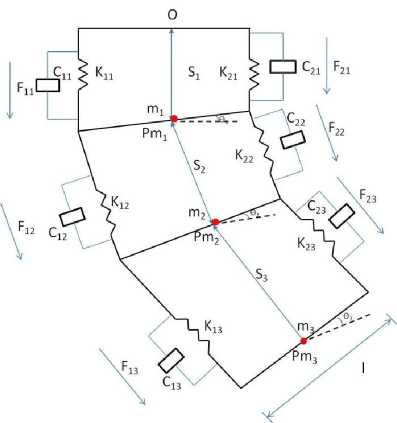
Fig. 1: Assumed structure for analytical model of a section of a continuum arm

Where;

I - Length of the rigid rod connecting the two struts, constant throughout the structure k,,t , i = 1,2,3 - Spring constant of actuator 1 at module k2,/ , i = 1,2,3  - Spring constant of actuator 2 at module

, ,  = 1,2,3 - Damping coefficient of actuator 1 at module

, ,  = 1,2,3 - Damping coefficient of actuator 2 at module

,  = 1,2,3 - Mass in each module

,  = 1,2,3 - Moment of inertia of the rigid rod in each module.

A global inertial frame (N) located at the base of the arm are given below

^P = S^

^p = s2. sind 1 ^ + (S1 + S2 cos 61). ^

тзР = (S2. sin01 + S3. sin(9 1 + 92)) ^

+ (Si

+

+ S3.cos(01 + 02 ))).^

The position vector of each mass is initially defined in a frame local to the module in which it is present. These local frames are located at the base of each module and oriented along the direction of variation of coordinate 's' of that module. The positioning of each of these masses is at the centre of mass of the rigid rods connecting the two actuators. Differentiating the position vectors we obtain the linear velocities of the masses. The kinetic energy (T) of the system comprises the sum of linear kinetic energy terms (constructed using the above velocities) and rotational kinetic energy terms due to rotation of the rigid rod connecting the two actuators, and is given below as т=(о.5)тг ̇/+(О.5) 7712 (( ̇ 28(116! + ̇ ч2 Z s2cos616^1)+( ̇1+ ̇ 2COS0! -

Szsindi ^̇ *1))+(о.5) ТПз (( ̇ 2Stn6! +

82СО89_г ^̇ ^1 + ̇ ₃sin(01 + 02)+

(  +   ) ̇  +      (  +  ) ̇

( ̇1+ ̇ 2СО8бг - S2Stn0! ̇ ^1 +

̇     (   +   )-      (   +   ) ̇

838т(61 + 02) ̇*2))+(о.5) 71 ̇

(О.5)^2 ( ̇>12 + ̇   )+(О.5)^з ( ̇'i2 +

̇ >22 + ̇ -з2).

The generalized forces in the system corresponding to the generalized co-ordinates are expressed as appropriately weighted combinations of the input forces.

$1 =    + ^ 21+( Г12 + F 22) cosOt +

( F13 + F 23) cos ( 9i + 9г )	(7)
Qs2 =    + F 22+( F13 + F 23) cos ( 9г )	(8)
Q$3 =    + ^23	(9)
Q61 =(1⁄2)( F11 - F21 )+(1⁄2)( F12 - F 22)+(1⁄2)( F13 - F 23)+ S2Stn02 (^13 + F 23)	(10)
Q61 =(1⁄2)( F12 - F22 )+(1⁄2)( F13 - F23 )	(11)
q91 =(1⁄2)( F13 - F23 )	(12)

The potential energy (P) of the system comprises the sum of the gravitational potential energy and the spring potential energy. A small angle assumption is made throughout the derivation. This allows us to directly express the displacement of springs and the velocities associated with dampers in terms of system generalized coordinates.

р=-mtgst - т2д(81 + S2COSdi)- т3д(81 + S2COS03 + S3COS(в^ + в^))+

(О.5) кц (S1+(1/2) 91 - Sc ⁾²+

(О.5)k₂i (S1+(1⁄2) 91 ^- 8 01)²⁺

(О.5)ki2 ( $2 +(1⁄2) 9г ^- 8 02 )²₊              (5)

(О.5)к₂2 ( $2 +(1⁄2) 9г - 8 02 )²+

(О.5)^13 (S3+(1⁄2) 9₃ ^- 8 03 )²+

(О.5)^23 (^s3+(1⁄2) 9₃ ^- 8 03 )²

where,S₀₁, *Sq2 , "Sq3 are the initial values of•Si , *^2 , iS^ respectively.

Due to viscous damping in the system, Rayliegh’s dissipation function [6] is used to give damping energy

It can be evinced from the force expressions that the total input forces acting on each module can be resolved into an additive component along the direction of extension and a subtractive component that results in a torque. For the first module, there is an additional torque produced by forces in the third module.

The model resulting from the application of Lagrange’s equations of motion obtained for this system can be represented in the form

Fcoeff X. =( q ) ̈ + c ( q ) ̇ + g ( q ⁾         (13)

where T is a vector of input forces and q is a vector of generalized co-ordinates. The force coefficient matrix ^coeff transforms the input forces to the generalized forces and torques in the system. The inertia matrix, D is composed of four block matrices. The block matrices that correspond to pure linear accelerations and pure angular accelerations in the system (on the top left and on the bottom right) are symmetric. The matrix c contains coefficients of the first order derivatives of the

D =(0.5) Сц ( ̇ 1 +(1/2) ̇*i)+

(0.5)C21 ( ̇1+(1/2) ̇*i)2+(0.5) c12 ( ̇2+

(1/2) ̇*2)+(0.5) C22 ( ̇2+(1/2) ̇*2) +      (6)

(0.5)c13 ( ̇3+(1/2) ̇*3)+(0.5) c23 ( ̇3+

(1/2) ̇*3).

= generalized co-ordinates. Since the system is nonlinear, many elements of c contain first order derivatives of the generalized co-ordinates. The remaining terms in the dynamic equations resulting from gravitational potential energies and spring energies are collected in the matrix G . The coefficient matrices of the dynamic equations are given below,

1	1	COS ( 9i)	cos ( 9i)	cos ( 9i + ^2 )	COS ( 9i + ^2 )
0	0	1	1	cos ( 02 )	cos ( 02 )
0	0	0	0	1	1	(14)
1⁄2	-1⁄2	1⁄2	-1⁄2	1⁄2+ s2sm ( 02 )	-1⁄2 + s2sm ( 02 )
0	0	1⁄2	-1⁄2	1⁄2	-1⁄2
0	0	0	0	1⁄2	-1⁄2     ⎦

D(я)=

c(я)=

⎡ ⎢ ⎢ ⎢ Сц + C21 ⎢ ⎢ ⎢ ⎢	-2 ^722^^^-( 9i) ̇ -2 ^Ti^sizi( 01 )6̇	-2 m3sin ( 9i + 02) ( t ̇ + I ̇ )	- m2s2 cos ( 61 )( t ̇ ) +(1⁄2)( Си + C21) - m3s2 cos (01)( t ̇ ) - m3s3 cos (01 + 62 )( t ̇ )	- m3s3stn ( 01 + 62 )	⎤ ⎥ ⎥ 0⎥ ⎥ ⎥ ⎥ ⎥
⎢ ⎢ ⎢ 0 ⎢ ⎢ ⎢ ⎢	C12 + ^22	-2 'n3si-n. ( 62 ) ( t ̇ + 6 ̇ )	- 1T13S3 ( t ̇ ) +(1⁄2) (C12 + C2 2 ) -m3s2 ( t ̇ ) - m3s3 cos ( 62 )( t ̇ )	-2 m3s3 cos ( e2 )( t ̇ ) - m3s3 cos (02)( t ̇ )	⎥ ⎥ ⎥ 0 ⎥ ⎥ ⎥ ⎥
⎢ ⎢ ⎢0 ⎢ ⎢	2m3sin( 62 )(6̇ )	C13 + C23	- m3s3s2 cos ( 62 )( t ̇ ) - 1T13S3 ( t ̇ )	-2m3s3 ( t ̇ ) - m3s3 ( t ̇ )	⎥ (1⁄2) (C13 + C23) ⎥ ⎥
⎢ ⎢ ⎢   (1⁄2) ⎢(Сц + ^21)	2m3s3 cos ( 62 )( t ̇ ) -2 m3s2 ( t ̇ ) +2 ^2S2 (t ̇ )	2m3s3 (6̇+6̇) -2m3s2 cos ( 92 ) (6̇+6̇)	2 m3s3s2 sin ( e2 )( t ̇ ) +(1 ⁄4) ( Сц + C21)	m3s3s2 sin ( 62 )( t ̇ )	⎥ ⎥ 0 ⎥ ⎥ ⎥
⎢ ⎢ ⎢ ⎢          0	(1⁄2)(Ci2 + c22)+ 2m3s3 cos ( 62 )( t ̇ )	2m3s3 (6̇+6̇)	m3s3s2 sin ( e2 )( 6 ̇ )	(1 ⁄4) (Ci2 + c22)	⎥ ⎥ 0           ⎥ ⎥
⎢ ⎣ ⎢        0	0	(1⁄2)(C13 - c23 )	0	0	(1 ⁄4)  ⎥ (C13 + C23)⎦

⎡    ml+ m2 ⎢+m3	m2cos ( 61 ) + m3cos ( 61 )	m3cos (0i + 02)	- m2s2sin ( 61 ) - m3s2sin ( 01 ) - m3s3sin ( 61 + 02)	- m3s3sin ( 61 + 6г )	0⎤	⎥⎥
⎢     m2cos (01) ⎢+ m3cos (01)	m2 + m3	m3cos (02)	- m3s3sin (02)	- m3s3sin (02)	0	⎥⎥
⎢ m3cos (01 + 02)	m3cos (02)	m3	m3s3sin (02 )	0	0	⎥⎥                   (15)
⎢ ⎢- m2s2sin (01) ⎢- m3s2sin (01) ⎢- m3s3sin ( 61 + 02)	- m3s3sin (02)	m3s2sin(02)	m2s2 + /i + /2 +/3 + m3s2 + m3si + 2m3s3cos ( 92) s2	^2 + m3si + ^3 + m3s3cos (02) S2		⎥ ⎥⎥
⎢ ⎢- m3s3sin ( 61 + 02) ⎢	- m3s3sin (02)	0	^2 + m3si + ^3 + m3s3cos (02) $11	^2 + m3si + ^3	^3	⎥ ⎥⎥ ⎥
⎣          0	0	0	^3	^3	/3⎦

c(я)=

• ^- miS - m₂g + fcn (Si + (1⁄2)61 - Soi)+ k₂i (Si - (1⁄2)6i - Soi)-m₃y ^⎡

⎢ ^- m₂gcos ( 61)+ к_г2 (S₂ + (1⁄2) e₂ - S₀2)+ k₂₂ (s₂ - (1⁄2) e₂ - S_O2)- m₃gcos ( 61 )

⎢- m₃gcos (61 + e₂ )+ ki₃ (s₃ +(1⁄2)0₃ - S₀3)+ k₂3 (S3 - (1⁄2)03 - S₀3 )

⎢ m2s2gsin(0i)+m3s3gsin( 0i + 02)+m3s2gsin(0i)+кц (Si + (1⁄2)0i - SOi)(1⁄2)

_⎢⎢                         ₊ к₂г (Si-(1⁄2)61 - Soi )(-1⁄2)

⎢

⎢ m₃s₃gsin ( 0i + ^2)+^12 (^S2 +(1⁄2)02 - ^S02)(1⁄2)+^22 (^S2 -(1⁄2)02 - ^S02)(-1⁄2)

⎣           кгз (s₃ + (1⁄2)03 - S₀3)(1⁄2) + k₂3 (S3-(1⁄2)03 - S₀3)(-1⁄2)

These dynamic formulations are very attractive from a control point of view.

• 2.2    Linear PD Main Controller

Design of a linear methodology to control of continuum robot manipulator was very straight forward. Since there was an output from the torque model, this means that there would be two inputs into the PD controller. Similarly, the outputs of the controller result from the two control inputs of the torque signal. In a typical PD method, the controller corrects the error between the desired input value and the measured value. Since the actual position is the measured signal. Figure 1 is shown linear PD methodology, applied to continuum robot manipulator [22-38].

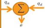
e (t) = 6_a(t) - 9_d(t)                                  (18)

Upd = K_Pa e + K_Vae                          (19)

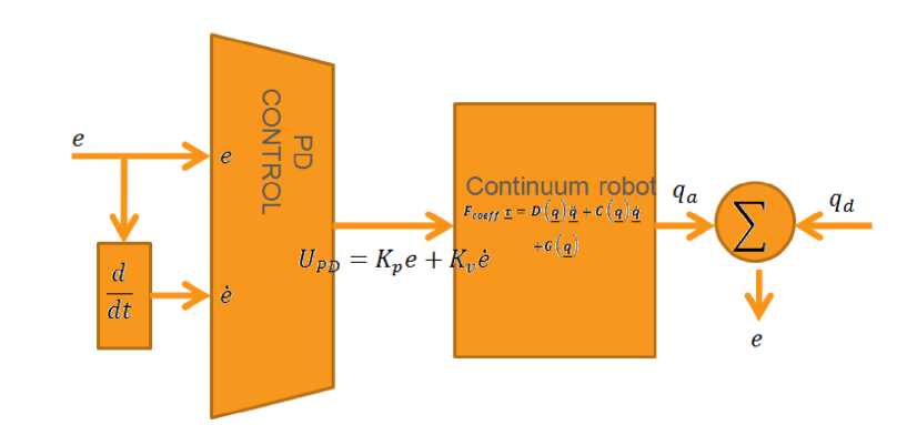
Fig. 1: Block diagram of linear PD method

The model-free control strategy is based on the assumption that the joints of the manipulators are all independent and the system can be decoupled into a group of single-axis control systems [18-23]. Therefore, the kinematic control method always results in a group of individual controllers, each for an active joint of the manipulator. With the independent joint assumption, no a priori knowledge of robot manipulator dynamics is needed in the kinematic controller design, so the complex computation of its dynamics can be avoided and the controller design can be greatly simplified. This is suitable for real-time control applications when powerful processors, which can execute complex algorithms rapidly, are not accessible. However, since joints coupling is neglected, control performance degrades as operating speed increases and a manipulator controlled in this way is only appropriate for relatively slow motion [44, 46]. The fast motion requirement results in even higher dynamic coupling between the various robot joints, which cannot be compensated for by a standard robot controller such as PD [47], and hence model-based control becomes the alternative.

x⁽ⁿ⁾ = f(x) + b( 5 r)u

Where u is the vector of control input, x⁽ⁿ⁾ is the n^th derivation of x, X= [x,x,x:,... ,X^(TI~ ¹⁾]^T is the state vector, f (x) is unknown or uncertainty, and b ( x) is of known sign function. The main goal to design this controller is train to the desired state;  x_d =

[x_d, Хд, X₄, ..^x^^{71 _ 1)}]^T, and trucking error vector is defined by [20-34]:

x = x - x_d = [x, . ,x^(n-1)]^T                      (21)

A time-varying sliding surface s(x, t) in the state space R ⁿ is given by [33]:

d s (x, t) = (— + Л)" 1 x = 0

where λ is the positive constant. To further penalize tracking error, integral part can be used in sliding surface part as follows [24-35]:

d .

s ⁽ x,t) = (-7- + Л) ^п-¹

2.3 Variable Structure Controller

Consider a nonlinear single input dynamic system is defined by [23-34]:

(!лд)

=

The main target in this methodology is kept the sliding surface slope s(x, t) near to the zero. Therefore,

one of the common strategies is to find input U outside of s(x, t) [24-33].

|^s2(x,t) <-<|s(x,t)| where ζ is positive constant.

If S(0)>0^S(t) <-<

U — -f + Хд - Л(Х - Xd)

A simple solution to get the sliding condition when the dynamic parameters have uncertainty is the switching control law [52-53]:

U dis — ^KtXtysgnts)

where the switching function sgn( S) is defined as [1, 6]

To eliminate the derivative term, it is used an integral term from t=0 to t=t_reac h

ft—treach Я            f

L d-'"'  '

^— breach

sgn ⁽s) — { li

-

s > 0

s < 0

s — 0

t=o

^S(t_reach)-S(O) < -'^(t reach ^- 0)

and the K(x, t) is the positive constant. Suppose by (24) the following equation can be written as,

Where t_{T each} is the time that trajectories reach to the sliding surface so, suppose S( t_{T eac}^ — 0) defined as;

0 - 5(0) <  -breach) ^ Г_теас11 <           (27)

and

Id, , „ „ s2 (x,t) — S^S

2 at

— [f - ^f - Ksgn(s)]

•5

— (f-f)^5-K|5|

and if the equation (28) instead of (27) the surface can be calculated as

sliding

if S (0) <0^0- 5(0) <  -breach) ^ 5(0) <  -(treach) .       . 1Я0)|

^ ^r reach <  _

s(x, t) — (5^ +^;i)² (/ x dr) — ⁽X - X d ) + 2Л(Х - X d )

Equation (28) guarantees time to reach the sliding surface is smaller than ^|5(0)| since the trajectories are outside of ( ) .

-

A² (x-x d )

in this method the approximation of is computed as [6]

if breach — ⁵⁽⁰⁾ ^ error(x - x_d) — 0      (29)

suppose S is defined as

^U — —^f + Хд — 2 Л(Х — X d )

+ A ²⁽ x-x d )

s (x, t) — (^ + A) x

= (x - Xd)

+ A(x - x d )

The derivation of S, namely, 5 can be calculated as the following;

5 = (X - X d ) + A(X - X d )

suppose the second order system is defined as;

x — f + и ^5 — f + U — Хд + A(x-x d )

Where is the dynamic uncertain, and also since 5 — 0 and 5 — 0, to have the best approximation , U is defined as

Based on above discussion, the variable structure control law for a multi degrees of freedom robot manipulator is written as [1, 6]:

U — Ue„ + Udis

Where, the model-based component      is the nominal dynamics of systems calculated as follows [1]:

Ueq — [D - 4 C+G ) + 5]O and     is computed as [1];

tens — K^sgn(S)

By (41) and (40) the variable structure control of robot manipulator is calculated as;

т — [D-4C + G) + 5]D + К • sgn(5)

where S = Л e + e in PD-SMC.

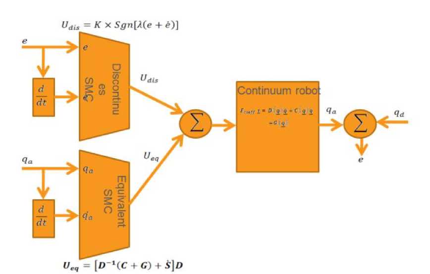
Fig. 2: Block diagram of nonlinear SMC compensator

2.4 Proof of Stability The lyapunov formulation can be written as follows,	By replacing the equation (48) in (43) V = ST(DS + C + G - DS+CS + G
1 V = —ST. D .S                             (43)	- Ks^n ( S) = ST (DS+CS + G          (49)
The derivation of V can be determined as,	- Ks^n(S)) and
У = ^ST.D.S + ST DS                    (44)	|DS+CS + G| < |DS| + |CS + G|           (50)
The dynamic equation of robot manipulator can be written based on the sliding surface as	The Lemma equation in CONTINUUM robot arm system can be written as follows
DS = -VS + DS + C + G               (45)	K „ = [|DS| + |CS + G|+4]  i
It is assumed that	= 1,2,3,4,^
ST (D + C + G)S = 0                    (46)	and finally;
by substituting (45) in (44)
1 V = -S t DS+CS + S t (dS + CS + G)     (47)	V <  - ^4 i |5 i |                             (52) i=l
= S t (dS + CS + G)	2.5 Fuzzy Logic Methodology
Suppose the control input is written as follows	Based on foundation of fuzzy logic methodology;
U = UNonhnear + U dts = [D-1(C+G) + S]D     (48) + K. s^n(S) + CS + G	fuzzy logic controller has played important rule to design nonlinear controller for nonlinear and uncertain systems [47]. However the application area for fuzzy control is really wide, the basic form for all command types of controllers consists of; Input fuzzification

(binary-to-fuzzy [B/F] conversion) Fuzzy rule base (knowledge base), Inference engine and Output defuzzification (fuzzy-to-binary [F/B] conversion). Figure 3 shows the fuzzy controller part.

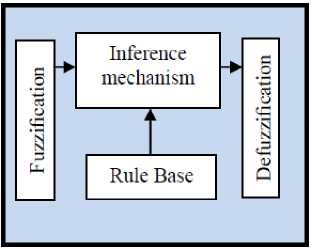
Fig. 3: Fuzzy Controller Part

The fuzzy inference engine offers a mechanism for transferring the rule base in fuzzy set which it is divided into two methods, namely, Mamdani method and Sugeno method. Mamdani method is one of the common fuzzy inference systems and he designed one of the first fuzzy controllers to control of system engine. Mamdani’s fuzzy inference system is divided into four major steps: fuzzification, rule evaluation, aggregation of the rule outputs and defuzzification. Michio Sugeno use a singleton as a membership function of the rule consequent part. The following definition shows the Mamdani and Sugeno fuzzy rule base [22-33]

if x is A and у is В then z is C 'ntamdani if x is A and у is В then z is f (x, y) 'sugeno'

When x and у have crisp values fuzzification calculates the membership degrees for antecedent part. Rule evaluation focuses on fuzzy operation (A ND / 0R ) in the antecedent of the fuzzy rules. The aggregation is used to calculate the output fuzzy set and several methodologies can be used in fuzzy logic controller aggregation, namely, Max-Min aggregation, Sum-Min aggregation, Max-bounded product, Max-drastic product, Max-bounded sum, Max-algebraic sum and Min-max. Defuzzification is the last step in the fuzzy inference system which it is used to transform fuzzy set to crisp set. Consequently defuzzification’s input is the aggregate output and the defuzzification’s output is a crisp number. Centre of gravity method ( C0 G ) and Centre of area method ( C0A ) are two most common defuzzification methods. Figure 4 shows fuzzy sliding mode compensator.

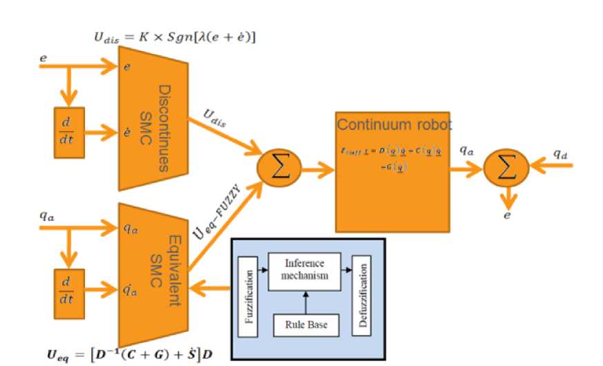
Fig. 4: Fuzzy logic estimator SMC

• III.    Methodology

Based on the dynamic formulation of continuum robot manipulator, (3), and the industrial PD law (5) in this paper we discuss about regulation problem, the desired position is constant, i.e., q^ = 0 . In most robot manipulator control, desired joint positions are generated by the trajectory planning. The objective of robot control is to design the input torque in (1) such that the tracking error

e = qd-qa (54)

When the dynamic parameters of robot formulation known, the PD control formulation (25) should include a compensator as

т=- к_ре - k_de +( G + F )               (55)

Where G is gravity and F is appositive definite diagonal matrix friction term (coulomb friction). If we use a Lyapunov function candidate as

^pd =¹ ̇ ^тм ̇+ е^тк_ре                   (56)

̇ pd =- ̇ ^тк_й ̇ ≤0                          (57)

Where П is a constraint set for 6 . For specific X , sup_{x ∈} и |/ ^ ₍ X | 9 ∗ _)-/( X )| is the minimum approximation error we can get.

We used the first type of fuzzy systems (58) to estimate the nonlinear system (26) the fuzzy formulation can be written:

f ( X | 9 )= 9^Т Е ( X )

∑      [ 9_ai ( х )]

=_∑Г=1 [ М-А¹ ( X )]

Based on above discussion ̇ =0 and е =0 are only initial conditions in Ω={[ ̇, е ]: ^̇ =0} , for which [ ̇, е ] ∈ Ω for al l t ≤0 . By the LaSalle^’s invariance principle, е →0 and с ̇ →0. When G and F in (25) are unknown, a fuzzy logic can be used to approximate them as

Where О¹ ,…, 9^й are adjusted by an adaptation law. The adaptation law is designed to minimize the parameter errors of 6 - 6 ^∗. The SISO fuzzy system is define as

/( X )= ⊖ ^Т Е ( X )

м

f ⁽ X )= ∑

Z = 1

9^l ℰ¹( X )= 9^Т ℰ( х )

Where

О =(0¹,…, 9^м ) т ,ℰ( х )=

(ℰ 1(X),…,ℰм(X))т, and ℰ1(X)= d.l(Х1)

:∏1=1 1 ∑ Г=1(∏?=1^(Xi)).      01,…,9м are adjustable parameters in (58). Цд1 (%1),…,На™ ( хи ) are given membership functions whose parameters will not change over time.

The second type of fuzzy systems is given by

/( X )=

^∑/ = 10' [∏7=1ехр(-( -   ))]

^∑ "•[∏ Ь ехр(-( - Л ))]

Where о¹ , a- and 8- are all adjustable parameters. From the universal approximation theorem, we know that we can find a fuzzy system to estimate any continuous function. For the first type of fuzzy systems, we can only adjust 6¹ in (59). We define / ^ ( X | 6 ) as the approximator of the real function/( X ).

f ^ ₍ X | 9 )= 9^те ( х )

We define 6 ^∗ as the values for the minimum error:

6 ^∗ =argmin

9 ∈ а

[sup|/ ^ ₍ х | 9 )- 9 ( х )|]

1-х ∈ U                                -I

Where

⊖ Т = (01,…, ^т )₌

г til ti² 0^м 1 “1 ^, “1 ,…, “1

⎢ ei ^, ol ,…, 9“ ⎥

⎣ 9L.919М ,   ,…,

£( х )=( Е¹ ( х ),…, Е^М ( X )) т , Е¹ ( X )=∏ ^^аХ ( Xi )/ ∑ ^=1(∏ ^l^ ( Xi )) , and M-_Ai. ( Xi ) is defined in (62). To reduce the number of fuzzy rules, we divide the fuzzy system in to three parts:

F¹ ( q , ̇)= ⊖ ^1T E ( q , ̇)

= *9^e (q, ̇) ,…,9m E (q, ̇) +

F² ( q , ̈ r )= ⊖ ^2T E ( q , ̈ r )

= *9^Te (q, ̈r) ,…,6m E (q, ̈r) +

F³ ( q , ̈)= ⊖ ^зТ E ( q , ̈)

= *9зТЕ (q, ̇) ,…,6m E (q, ̈) +

The control security input is given by

T=      ̈  + C ( q ) ̇²+ 9 ( q )+

F1 (q, ̇)+ F2 (q, ̈ )+ F3 (q, ̈)- Kpe -

̇

Where D ^{^} , C ( q ) ̇'² , g ( q ) are the estimations of D ( q ).

Based on sliding mode formulation (42) and PD linear methodology (19);

^New =((̇+Лб)

And ^switch is obtained by

Uswitch =K( ⃗ х ⃗ , t) ∙sgn(SNew) =K( ⃗ х ⃗ , t)∙ sgn ( К ((̇+Ле))

The Lyapunov function in this design is defined as

м

1   11

^v=₂ STMS +₂∑ Ysj^ ^. Ф,              (71)

where Ysj is a positive coefficient, Ф=  ∗-3,3∗ is minimum error and 6 is adjustable parameter. Since ̇-2 is skew-symetric matrix;

S^TD< ̇+ S^TL ^̇ 'S =   ( D‘ ̇+ VS )              (72)

If the dynamic formulation of robot manipulator defined by т=(q) ̈+v(q, ̇) ̇+g(q)

The controller formulation is defined by

T= ^̂ ̈ + ^̂ ̇ + ^̂- AS - К

According to (72) and (73)

D(q) ̈+v(q, ̇) ̇+G(q)= ̂ ̈ + ̂ ̇ + ̂--

Since ̇  = ̇- and ̈  =̈-

DS ^̇+( v + A ) S =∆ f - К

̇=   -  --

The derivation of V is defined

̇=     ̇+1   ̇  +∑1

²              Ysj

M

^̇= S^T ( D ^̇+ VS )+∑ — ф^т . ^̇

Ysi

/=1

Based on (75) and (76)

V̇=ST(Δf-K-VS-λS+VS)+

∑j=i — nT. ̇ γ where           ∆f=[D(q) ̈+v(q, ̇) ̇+G(q)]-

∑ Y=i9^T^ ( X )

̇=∑[ (  -  )]-    +∑    . ̇

Suppose Kj is defined as follows

• (73)

• (74)

• (75)

• (76)

• (77)

• (78)

_K = ^∑ ?j^l ^[ ЦА ⁽ Sj )] _{= 6}T< (_s ) =_∑ [ Ha ( Sj )] ⁼ е,⁽Sj⁾

where ^j ⁽ Sj )=[ Q ⁽ Sj ), ^j ⁽ Sj ), ^i ⁽ Sj ), ….. ^, ^j ⁽ Sj )]^r

⁽ Sj )=

±( A ) j ⁽ Sj ^{) ∑} iH ( A ) ' ( Sj )

where M- ( xi ) is membership function. The fuzzy system is defined as

∑

9^T^ ( x )= ^(e, ̇)    (81)

where 9=(01, 02, 93,…….,9м)   is adjustable parameter in (79)

According to (76), (77) and (79);

̇=∑ J=i [ Sj (Δ /i ^- 0^T<( Sj )]- S^TAS +

∑   ∑     . ̇            ( )           +

Based on Ф= ∗-0→0=

V̇=

^∑J=1 [S i(Δf-θ ^∗ T ζ(Si)+

□Tζ(S j )]-STλS+∑M i—   . ̇

γ

̇=∑[ (   -( ∗) ()]-

7=1M

+∑      [  .  .  ( )+])

where ^̇ fy =        ( Sy) is adaption law , ∅ ^̇₇=- ^{̇ =}

- YsjSj^j ( Sj ) ^̇ is considered by

̇=∑[ ∆ -(( ∗)  ( ))]-

The minimum error is defined by

^mj =∆fj-((6 ∗) T^j ( Sj))

Therefore ̇ is computed as

̇=∑[Sj emj]-STAS(86)

≤∑ £ | Sj || ^mj |- S^TAS

=∑| Sj || 6m j |- AjSj² i=i

т

= 2^l(lewl-^)              (87)

7 = 1

For continuous function g(x), and suppose e > 0 it is defined the fuzzy logic system in form of

SupxeylfOc) - g(x)| < e                     (88)

The minimum approximation error (e_mj) is very small.

if Aj = a t^a t  a|Sj| > emj (S j ^

0)    t^en  V < 0 fо r (Sj ^ 0)

я^Н^-^^ я 1₁ |п_Г„=х, ⁽ -( ^)^{2 )} |

Kaei)

x(     +

The different between PDxSMC and PDxSMC+FL is uncertainty. In PDxSMC the uncertainty is d = G + F + f . The sliding mode gain must be bigger than its upper bound. It is not an easy job because this term includes tracking errors e_г and q _г. While in PDxSMC+FL, the uncertainty η is the fuzzy approximation error for G + F + f .

This method has two main controller’s coefficients, . To tune and optimize these parameters mathematical formulation is used

G+F+f=

^ ₁₆jn i _{1 6} xp (- (^) )+ ^ !■ 1^(-^)²)]

u = (ufuzzy + UsUdlng) x UPD                (90)

U = Ufuzzy + Uwitch) X Upd =

[D"1 (B + C + G) + S]D + К • s gn(S) +

It is usually is smaller than G + F + f ; and the upper bound of it is easy to be estimated. Figure 5 shows the PD controller with serial PD fuzzy sliding mode controller.

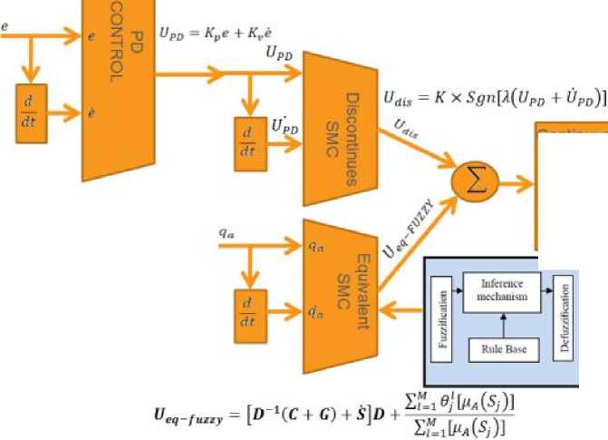
.il.i ;,

Fig. 5: PD with fuzzy SMC Compensator

Continuum robo

o a a-c s 5

• IV.    Results and Discussion

Linear PD controller (PD) and proposed PD with SISO fuzzy sliding mode estimator were tested to sinus response trajectory. The simulation was implemented in MATLAB/SIMULINK environment. Links trajectory and disturbance rejection are compared in these controllers. It is noted that, these systems are tested by band limited white noise with a predefined 40% of relative to the input signal amplitude. This type of noise is used to external disturbance in continuous and hybrid systems.

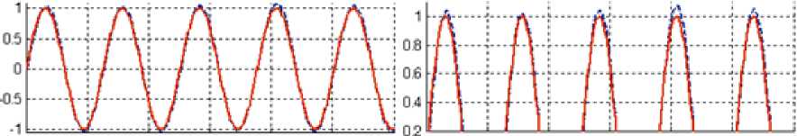
Trajectory: Figure 6 shows the links trajectory in PD controller and proposed PD with SISO fuzzy variable structure estimator without disturbance for sinus trajectory in general and zoom scaling because all 3 joints have the same response so, all links are shown in a graph.

PD

Proposed

0       5      10      15      20      25      30 0       5      10      15      20      25      30

Fig. 6: PD controller Vs. Proposed method

By comparing sinus response, Figure 6, in PD controller and PD with FSMC estimator, we can seen the the proposed controller’s overshoot (0%) is lower than PD's (7.8%) .

Disturbance rejection: Figure 7 is indicated the power disturbance removal in PD controller and PD with SISO

FSMC estimation. Besides a band limited white noise with predefined of 40% the power of input signal is applied to the sinus PD controller and proposed method; it found slight oscillations in PD trajectory responses. All 3 joints are shown in one graph.

PD

Proposed

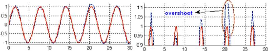
Fig. 7: PD Vs. Proposed method: Robot arm with external disturbance

Among above graph, relating to sinus trajectory following with external disturbance, PD controller has slightly fluctuations. By comparing overshoot; proposed controller's overshoot (1.3%) is lower than PD's (22%).

improved by using the advantages of sliding mode methodology and artificial intelligence compensate while the disadvantages removed by added each method to previous method.

• V.    Conclusion

Refer to the research, a Lyapunov based SISO fuzzy sliding mode estimator PD controller design and application to continuum robot arm has proposed in order to design high performance nonlinear estimator in the presence of highly uncertainties and external disturbances. Regarding to the positive points in linear PD controller, sliding mode controller and fuzzy inference system it is found that the fuzzy logic laws derived in the Lyapunov sense. The stability of the closed-loop system is proved mathematically based on the Lyapunov method. The first objective in proposed method is removed the chattering based on artificial intelligence. The second target in this work is compensating the model uncertainty by SISO fuzzy inference system, in the case of continuum robot arm. In finally part fuzzy sliding mode methodology with minimum rule base is used to compensate and adjusted the PD controller. In this case the performance is