Design Stable Robust Intelligent Nonlinear Controller for 6- DOF Serial Links Robot Manipulator

Published Online July 2014 in MECS DOI: 10.5815/ijisa.2014.08.03

System or plant is a set of components which work together to follow a certain objective. Based on above definition, in this research robot manipulator is system. A robot is a machine which can be programmed to do a range of tasks. They have five fundamental components; brain, body, actuator, sensors and power source supply. A brain controls the robot’s actions to best response to desired and actual inputs. A robot body is physical chasses which can use to holds all parts together. Actuators permit the robot to move based on electrical part (e.g., motors) and mechanical part (e.g., hydraulic piston). Sensors give robot information about its internal and external part of robot environment and power source supply is used to supply all parts of robot. Robot is divided into three main groups: robot manipulator, mobile robot and hybrid robot. Robot manipulator is a collection of links which connect to each other by joints. Each joint provides one or more Degrees Of Freedom (DOF). Figure Robot manipulator is divided into two main groups, serial links robot manipulator and parallel links robot manipulators. In serial or open-chain links robot manipulator, links and joints is serially connected between base and final frame (end-effector). Parallel or closed-chain robot manipulators have at least two direction between base frame and end-effector. Serial link robot manipulators having good operating characteristics such as large workspace and high flexibility but they have disadvantages of low precision, low stiffness and low power operated at low speed to avoid excessive vibration and deflection. However the advantages of parallel robot manipulator are large strength-to-weight ratio due to higher structural rigidity, stiffness and payload they have disadvantage such as small workspace. Study of robot manipulators is classified into two main subjects: kinematics and dynamics. The study between rigid bodies and end-effector without any forces is called Robot manipulator Kinematics. Study of this part is very important to design controller and in practical applications. The study of motion without regard to the forces (manipulator kinematics) is divided into two main subjects: forward and inverse kinematics. Forward kinematics is a transformation matrix to calculate the relationship between position and orientation (pose) of task (end-effector) frame and joint variables. This part is very important to calculate the position and/or orientation error to calculate the controller’s qualify. Forward kinematics matrix is a 4x4 matrix which 9 cells are show the orientation of end-effector, 3 cells show the position of end-effector and 4 cells are fix scaling factor. Inverse kinematics is a type of transformation functions that can used to find possible joints variable (displacements and/or angles) when all position and orientation (pose) of task be clear [1-3]. Figure 1 shows the application of forward and inverse kinematics. A dynamic function is the study of motion with regard to the forces. Dynamic modeling of robot manipulators is used to illustrate the behavior of robot manipulator (e.g., nonlinear dynamic behavior), design of nonlinear conventional controller (e.g., conventional computed torque controller, conventional sliding mode controller and conventional backstepping controller) and for simulation. It is used to analyses the relationship between dynamic functions output (e.g., joint motion, velocity, and accelerations) to input source of dynamic functions (e.g., force/torque or current/voltage). Dynamic functions is also used to explain the some dynamic parameter’s effect (e.g., inertial matrix, Coriolios, Centrifugal, and some other parameters) to system’s behavior [3].

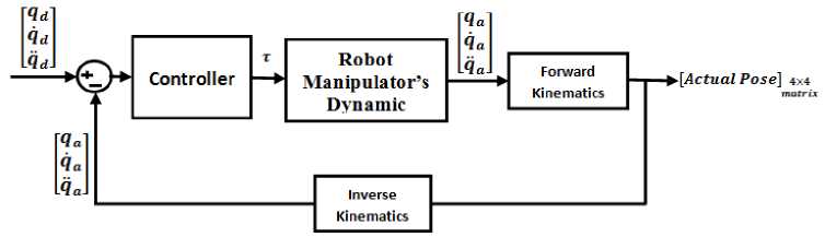
Fig. 1. The application of Forward and Inverse Kinematics

Automatic control has played an important role in advance science and engineering and its extreme importance in many industrial applications, i.e., aerospace, mechanical engineering and robotic systems. The first significant work in automatic control was James Watt’s centrifugal governor for the speed control in motor engine in eighteenth century[2]. There are several methods for controlling a robot manipulator, which all of them follow two common goals, namely, hardware/software implementation and acceptable performance. However, the mechanical design of robot manipulator is very important to select the best controller but in general two types schemes can be presented, namely, a joint space control schemes and an operation space control schemes[1]. Joint space and operational space control are closed loop controllers which they have been used to provide robustness and rejection of disturbance effect. The main target in joint space controller is design a feedback controller that allows the actual motion ( qa (t) ) tracking of the desired motion ( qd(t) ). This control problem is classified into two main groups. Firstly, transformation the desired motion Xd (t) to joint variable Я a (t) by inverse kinematics of robot manipulators [4-6]. The main target in operational space controller is to design a feedback controller to allow the actual endeffector motion ( ) to track the desired endeffector motion Xd(t) . This control methodology requires a greater algorithmic complexity and the inverse kinematics used in the feedback control loop. Direct measurement of operational space variables are very expensive that caused to limitation used of this controller in industrial robot manipulators[6-8]. One of the simplest ways to analysis control of multiple DOF robot manipulators are analyzed each joint separately such as SISO systems and design an independent joint controller for each joint. In this methodology, the coupling effects between the joints are modeled as disturbance inputs. To make this controller, the inputs are modeled as: total velocity/displacement and disturbance. Design a controller with the same formulation and different coefficient, low cost hardware and simple structure controller are some of most important independent-joint space controller advantages. Nonlinear controllers divided into six groups, namely, feedback linearization (computed-torque control), passivity-based control, sliding mode control (variable structure control), artificial intelligence control, Lyapunov-based control and adaptive control[9-17].

One of the robust nonlinear controllers which have been analyzed by many researchers especially in recent years to control of robot manipulator is sliding mode controller (SMC). Sliding mode controller (SMC) is robust conventional nonlinear controller in a partly uncertain dynamic system’s parameters. This conventional nonlinear controller is used in several applications such as in robotics, process control, aerospace and power electronics. This controller can solve two most important challenging topics in control theory, stability and robustness [ 18-22]. The main idea to design sliding mode control is based on the following formulation;

_ (Tt ⁽q, t)  if S i > 0

^(q, ^t) (T f (q, t)   if S_i< 0

where S_i is sliding surface (switching surface), i = 1,2,......,n for n -DOF robot manipulator, t( q, t) is the i^th torque of joint. According to above formulation the main part of this control theory is switching part this idea is caused to increase the speed of response. Sliding mode controller is divided into two main sub parts:

• •    Discontinues controller(T j _is)

• •    Equivalent controller(T_e q )

Figure 2 shows the main part of sliding mode controller with application to serial links robot manipulator.

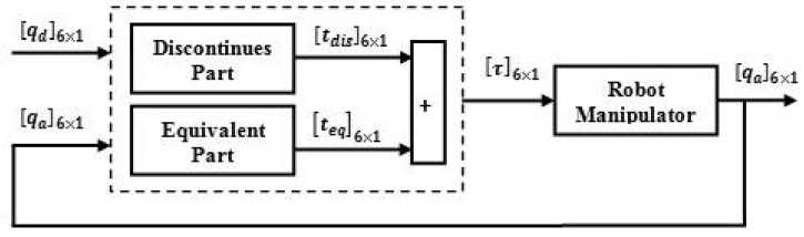
Fig. 2. Block diagram of Conventional Sliding Mode Controller

Discontinues controller is used to design suitable tracking performance based on very fast switching. This part of controller is work based on the linear type methodology; therefore it can be PD, PI and PID. Fast switching or discontinuous part have essential role to achieve to good trajectory following, but it is caused system instability and chattering phenomenon. Chattering phenomenon is one of the main challenges in conventional sliding mode controller and it can causes some important mechanical problems such as saturation and heats the mechanical parts of robot manipulators or drivers. Equivalent part of robust nonlinear sliding mode controller is the impact of nonlinear term of serial links robot manipulator. It is caused to the control reliability and used to fine tuning the sliding surface slope [3- 7]. The equivalent part of sliding mode controller is the second challenge in uncertain systems especially in robot manipulator because in condition of uncertainty calculate the nonlinear term of robot manipulator’s dynamic is very difficult or unfeasible. The formulations of sliding mode controller with application to six degrees of freedom serial links robot manipulator is presented based on [3- 7].

However, conventional sliding mode controller is used in many applications such as robot manipulator but, this controller has two main challenges [22]:

• •    chattering phenomenon

• •    nonlinear equivalent dynamic formulation in uncertain parameters

Based on the literature to reduce or eliminate the chattering, various papers have been reported by many researchers which classified into two main methods:

• •    boundary layer saturation method

• •    artificial intelligence based method

The methodology of boundary layer saturation method is achieve accurate tracking for non-linear and time varying system in presence of disturbance and parameter variations based on continuous feedback control law. Slotine and Sastry design conventional switching sliding mode controller for nonlinear system in presence of uncertainty and external disturbance. To rectify the chattering phenomenon, the saturation continuous control is introduced [19]. Slotine is presented sliding mode controller for nonlinear system [20]. According to [20] he solved the chattering challenges based on linear boundary layer method to improve the industry applications.

Saturation boundary layer method has some disadvantages such as increase the error and reduces the speed of response. To solve linear boundary layer saturation challenge Palm [21] design nonlinear intelligent saturation boundary layer function instead of linear saturation boundary method. This method is used to reduce or eliminate the chattering as well as reduce the error performance. In this design the fuzzy controller has two inputs and has 49 rule bases. However the design sliding mode fuzzy controller to reduce the chattering is faster and robust than sliding mode controller based on linear boundary layer method but adjust the fuzzy logic input and output gain updating factor is very difficult.

The chattering phenomenon may be eliminated by linear boundary layer method but there is no theoretical Lyapunov stability proof for using this control law.

Based on the following literature to solve the equivalent challenge in presence of uncertainty and external disturbance, various papers have been reported by many researchers which classified into two main methods:

• •    design fuzzy sliding mode controller

• •    design sliding mode fuzzy controller

Fuzzy sliding mode controller (FSMC) is robust nonlinear intelligent controller. In this methodology the main controller is sliding mode controller and fuzzy logic controller is applied to it to estimate the nonlinear dynamic formulation in presence of uncertainty and external disturbance. Wu et al. [22] have proposed a PI sliding mode controller with fuzzy logic tuning controller for Electro-Hydraulic Driving. In this research authors first of all design PI sliding mode controller based on switching function and equivalent dynamic equations and after that design fuzzy logic estimator that design parallel with PI sliding mode controller to estimate the nonlinear equivalent functions. In this design the chattering phenomenon is reduced but in presence of uncertainty it has chattering. Barrero. et. al [23] have proposed a fuzzy supervisory controller for fuzzy sliding mode controller to reduce above challenge with application to induction motor. In this design PI fuzzy logic controller is applied to sliding mode methodology to reduce the chattering as well as improve the equivalent nonlinear dynamic formulation to modify the transient and steady state response based on the 25 fuzzy rule bases. To improve the output result supervisory fuzzy controller with 9 rule bases used to on line tuning the sliding mode and PI fuzzy logic parameters. However above method have two fuzzy logic controls for system estimation and on line tuning the parameters but it cannot eliminate the torque chattering phenomenon which caused to heating in system mechanical parameters. To improve above challenge Shahnazi,et.,al [24] design adaptive fuzzy PI sliding mode controller for induction motor. To improve the chattering phenomenon as well as nonlinear dynamic equivalent parameters PI fuzzy sliding mode is designed. Adaptive supervisory controller is applied to antecedent and consequent part of fuzzy logic controller to estimate and online tuning especially in presence of uncertainty.

Sliding mode fuzzy controller (SMFC) is a robust intelligent based controller. In this controller the main controller is fuzzy logic controller and sliding mode controller is applied to fuzzy logic controller to reduce the fuzzy rules based on reduce the number of inputs and improve the stability of close loop system in fuzzy logic controller [21, 25-28]. Weng and Yu [29] design sliding mode fuzzy controller to reduce the number of rule base in pure fuzzy logic controller and improve the stability. In this research the adaptive methodology was used to online tune the fuzzy parameters to reduce the chattering phenomenon. According to above discussion the fuzzy logic controller in this research has one input (S) and one output therefore the number of rule base is reduce compare to fuzzy sliding mode methodology. To improve the sliding surface boundary layer thickness Lhee et al. [26] have presented a sliding mode fuzzy logic controller. According to this research sliding mode controller caused to improve the robust and fuzzy logic controller is used to fast speed change the boundary layer thickness in uncertain condition to reduce the chattering around the sliding surface. In above two researches, the fuzzy input was (S) that it can be Proportional plus Derivative (P+D) or Proportional plus Integral (P+I) or Proportional plus Integral plus Derivative (P+I+D), therefore in these entire design fuzzy logic controller have one complex input. Zhang et al. [28] design sliding mode fuzzy controller to improve the resistance to the external disturbance and reduce the chattering phenomenon. Based on this research the fuzzy logic controller has two inputs that the first one was sliding surface and the second one was self tuning mechanism function. In comparison, to reduce the number of fuzzy rule base, increase the robustness and stability sliding mode fuzzy controller is more suitable than fuzzy logic controller [28]. In comparison between sliding mode fuzzy controller and fuzzy sliding mode controller it can seen that, sliding mode fuzzy controller has two important drawbacks namely:

• •    High sensitivity to  the  sliding surface slope

coefficient.

• •    Challenge in design and implementation which fuzzy sliding mode controller is more suitable for implementation.

According to classical nonlinear control theory such as sliding mode controller or computed torque controller, these types of controllers are worked based on manipulator dynamic model. Based on equivalent part in conventional nonlinear controllers, in complex and highly nonlinear systems these controllers have many problems for accurate response. Conventional nonlinear controllers need to have accurate knowledge of dynamic formulation of system and it is one of the main challenges. In recent years, artificial intelligence theory has been used in control of nonlinear systems. In most of research papers, neural network, fuzzy logic and neuro-fuzzy are used in nonlinear, time variant and uncertain systems (e.g., robot manipulator) for system identification and control. Fuzzy logic controller (FLC) is one of the most important applications of fuzzy logic theory. This controller can be used to control of nonlinear, uncertain, and noisy systems. After the invention of fuzzy logic theory in 1965 by Zadeh, this theory was used in wide range applications such as control theory or system modeling. The nonlinear dynamic formulation problem in highly nonlinear system (e.g., robot manipulator) can be solved by fuzzy logic theorem. Fuzzy logic theory is used to estimate the system dynamics. This type of controller is free of mathematical dynamic parameters of plant.

The basic fuzzy controller to control of two degrees of freedom was presented in 2002 by Zhou and Coiffet [32]. In this paper dynamic and kinematics part of robot controlled and modified by two inputs fuzzy logic controller based on 25 rule bases. According to this research the first link error is bigger than the second link and this controller is not reliable, because it is model free. Design fuzzy logic for two degrees of freedom robot manipulator was introducing by Banerjee and Woo [33]. In this paper Mamdani fuzzy inference system based on 49 rule bases was design and analyzed. This controller was nonlinear model free and the main challenges in this design is reliability and this item is one of the most important part to select the best method of control design.

An Important question which comes to mind is that why this proposed methodology should be used when lots of control techniques are accessible?

The dynamics of a robot manipulator is highly nonlinear, time variant, MIMO, uncertain and there exist strong coupling effects between joints. The problem of coupling effects can be reduced, with the following two methods:

• •    Limiting the performance of the system according to the required velocities and accelerations, but now the applications demand for faster and lighter robot manipulators.

• •    Using a high gear ratio (e.g., 250 to 1) at the mechanical design step, in this method the price paid is increased due to the gears.

Therefore linear type of controller, such as PD or PID cannot be having a good performance. Consequently, to have a good performance, linearization and decoupling without using many gears, feedback linearization (computed-torque) control methodologies can be presented. In order to design computed torque controller, an accurate dynamic model of robot manipulator plays an important role. To modelling an accurate dynamic system, modelling of complex parameters is needed to form the structure of system’s dynamic model. It may be very difficult to include all the complexities in the system dynamic model. Dynamic parameters may not be constant over time; subsequently adaptation methodology plays a vital role. System’s dynamic parameter estimation in computed torque-based adaptive control methodology can be realized if acceleration term should be measured, but this work is very expensive. Furthermore, PUMA robot manipulator dynamic models through    a large number of highly nonlinear parameters generate the problem of computation as a result it is caused to many challenges for real time applications. To eliminate the actual acceleration measurement and also the computation burden as well as have stabile, efficiency and robust controller, sliding mode controller is introduced. Assuming unstructured uncertainties and structure uncertainties can be defined into one term and considered as an uncertainty and external disturbance, the problem of computation burden and large number of parameters can be solved to some extent. Now the most important target in this part is reducing the uncertainties limitation and assures the asymptotic stability for large area possible circumstances. The main method to solve this problem based on Gutman methodology is: if the bounds of lumped uncertainty are incorporated to build the control law then it can· be shown that asymptotic stability is assured in the presence of uncertainties [34]. Hence conventional switching sliding mode controller is an apparent nominates to design a controller using the bounds of the uncertainties and external disturbance. Based on literature there are three main issues limiting the applications of conventional sliding mode controller; equivalent part related to dynamic equation of robot manipulator, computation of the bounds of uncertainties and chattering phenomenon. The problem in equivalent nonlinear dynamic formulation of robot manipulator is not a simple task and fuzzy logic theory is used to reduce this challenge. If PD+I fuzzy logic controller is used, we have limitation in the number of fuzzy rule table. Uncertainties are very important challenges and caused to overestimation of the bounds. As this point if S = Kie + e + K£e = 0 is chosen as desired sliding surface, if the dynamic of robot manipulator is derived to sliding surface and if switching function is used to reduce the challenge of uncertainty then the linearization and decoupling through the use of feedback, not gears, can be realized. Because, when the system dynamic is on the sliding surface and switching function is used the derivative of sliding surface S = Kie + e + K2e is equal to the zero that is a decoupled and linearized closed-loop PUMA robot dynamics that one expects in computed torque control. Linearization and decoupling by the above method can be obtained in spite of the quality of the robot manipulator dynamic model, in contrast to the computed-torque control that requires the exact dynamic model of a system. It is well known fact that if the uncertainties are very good compensate there is no need to use discontinuous part which create the chattering. To compensate the uncertainties fuzzy logic theory is a good candidate, but design a fuzzy controller with perfect dynamic compensation in presence of uncertainty is very difficult. Therefore, if the uncertainties are estimated and if the estimation results are used by discontinuous feedback control, and if linear part controller is added to this part, chattering can be eliminated. Finally, for a linear and partially decoupled dynamics of the robot manipulator, when the result is near to the sliding surface, a linear controller is designed based on the deviation of state trajectories from the sliding surface.

This paper is organized as follows; second part focuses on the modeling dynamic formulation based on Lagrange methodology, fuzzy logic methodology and sliding mode controller to have a robust control. Third part is focused on the methodology which can be used to reduce the error, increase the performance quality and increase the robustness and stability. Simulation result and discussion is illustrated in forth part which based on trajectory following and disturbance rejection. The last part focuses on the conclusion and compare between this method and the other ones.

• I I. T heory

Dynamic and Kinematics Formulation of 6DOF Serial Links Robot Manipulator:

System Kinematics: In this research to forward kinematics is used to system modeling. Wu has proposed PUMA 560 robot arm forward kinematics based on accurate analysis [4]. The main target in forward kinematics is calculating the following function:

V(X,q) = 0                             (2)

Where ^ (.) £ Fn is a nonlinear vector function, X = [Xi,X2,......,Xl]T is the vector of task space variables which generally endeffector has six task space variables, three position and three orientation, q = [qi, q2, ...., qn]T is a vector of angles or displacement, and finally n is the number of actuated joints.

Calculate robot manipulator forward kinematics is divided into four steps as follows;

• •    Link descriptions

• •    Denavit-Hartenberg (D-H) convention table

• •    Frame attachment

• •    Forward kinematics

The first step to analyze forward kinematics is link descriptions. This item must to describe and analyze four link and joint parameters. The link description parameters are; link length (a / ) , twist angle («), link offset (d / ) and joint angle (6 / ). Where link twist, is the angle between Z^ and Z / _+i about an X / , link length, is the distance between Z / and Z / _+i along X / and d / , offset, is the distance between X /_ _i and X / along Z / axis. In these four parameters three of them are fixed and one of parameters is variable. If system has rotational joint, joint angle (6 / ) is variable and if it has prismatic joint, link offset (d / ) is variable.

The second step to compute Forward Kinematics (F.K) of robot manipulator is finding the standard D-H parameters. The Denavit-Hartenberg (D-H) convention is a method of drawing robot manipulators free body diagrams. Denvit-Hartenberg (D-H) convention study is compulsory to calculate forward kinematics in robot manipulator. Table 1 shows the standard D-H parameters for N-DOF robot manipulator. Figure 3 shows the D-H notation of research’s plan (PUMA robot manipulator).

Table 1. The Denavit Hartenberg parameter

Link i	0 i (rad)	a , (rad)	a , (m)	d , (m)
1	6 i	« i	ai	di
2	62	« 2	a2	d2
3	6 3	« 3	a3	d3
........	......	.......	.......	........
........	.......	.......	........	........
N	6 „	n	as	d n

The third step to compute Forward kinematics for robot manipulator is finding the frame attachment matrix. The rotation matrix from {F / } to {F /_ _i} is given by the following equation;

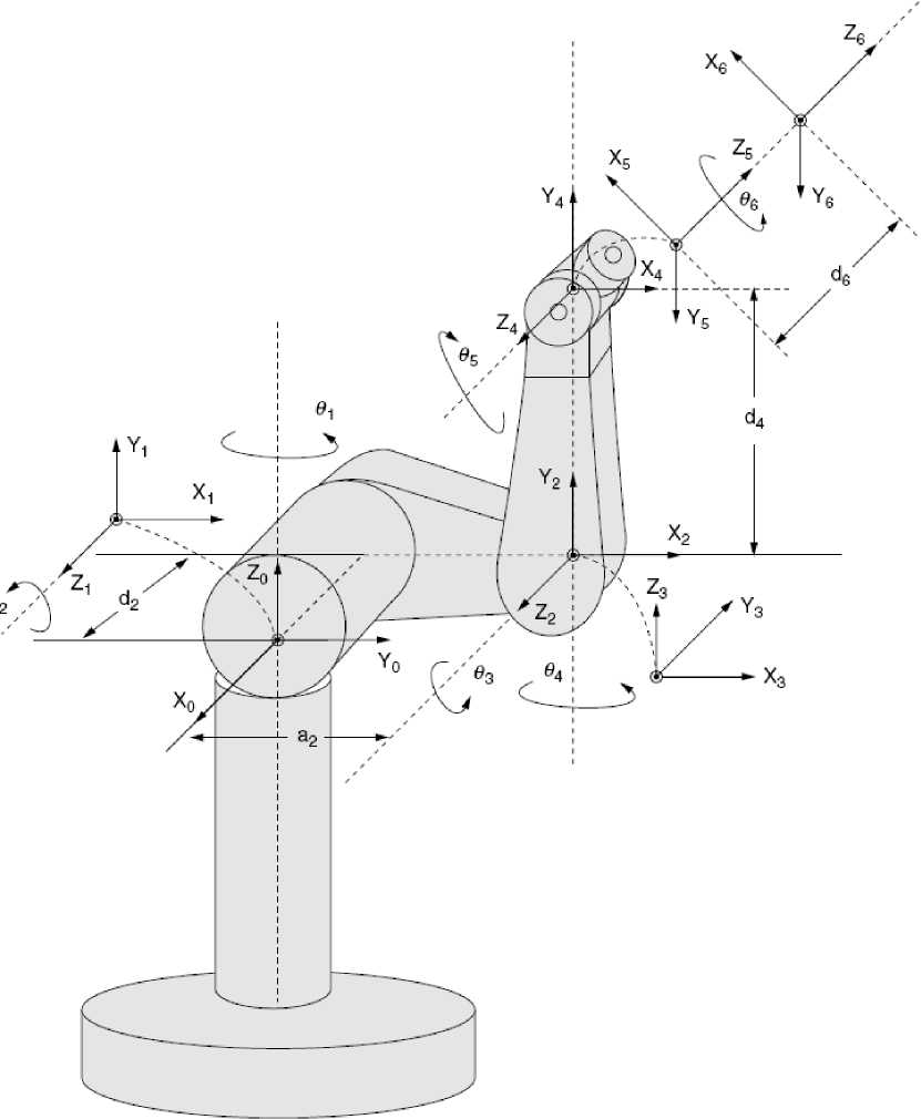
Fig. 3. D-H notation PUMA robot manipulator[5]

R Г ¹ = u_K6t )V_Kai )

Where U^g^ is given by the following equation [3];

Ul W)

cos (6^  -sin(6t)0

sin (6i)   cos(6i)0

0        01

and V /(_a.) is given by the following equation [3];

1     0.

V i(6_i) = I^{0   os}s(ad

0  sin(ai)

-sin(a i ) cos(a i )

So (R ° ) is given by [3]

R£ = (U1V1)(U2V2).........(U„V„)(6)

n-iT _ [Rn-1d

"r"l 0     1 1

The transformation (frame attachment) matrix is compute as the following formulation;

=
" COt	- SOt	0	^i —1
S6t Cai_1	С6( Cai_1	- Sai_1	- Stti-^t
S6t Sai_1	С6( Sai_1	Cai_1	C«i-idi
0	0	0	1

The forth step is calculate the forward kinematics by the following formulation [3]

FK _ От _ O'T’ l»p 2^ п-1т _

=   =   ․ 21 ․ 3' ……․=

[ О 1" ]=   ․   ․   ……․=

Bx =- sin ( 9ь ) × ( cos ( 9s ) ×

(cos (9*) × cos(9г + 93) × cos(9i) + sin(9i) × sin(9i)) + sin(9s) × sin(92 + @3) × cos (9i))+cos (9b)×

(sin(9i)×cos (92 + 93)×cos (9i)- cos(9i)×sin(9i))

By =- sin ( 9_b )×( cos ( 9s )×( cos ( 9i )× cos ( 9₂ + 9з )× sin ( 9i )- sin ( 9i )× cos ( 9i )) + sin ( 9₅ )× sin ( 9₂ + 9з ) × sin ( 9i )) + cos ( 9 b )×( sin ( 9i )×           (15)

cos ( 9_г + 9₃ )× sin ( 9i )+ cos ( 9i )× cos ( 9i ))

Based on above formulation the final formulation for PUMA robot manipulator is;

"N_x B_x T_x P_x ^У By Ту Py N_z B_z T_z P_z

.0 0 0 1.

Bz =- sin ( 9_b )×( cos ( 9s )× cos ( 9i )× sin ( 9₂ + 9₃ )- sin ( 9s )× cos ( 9₂ + 9₃ ))+ cos ( 9₆ )× sin ( 9i )× sin ( 9₂ + 9₃ )

Tx =   ( 9з )×( cos ( 9i )× cos ( 9₂ +

9з )× cos ( 9i )+ sin ( 9i )× sin ( 9i ))- cos ( 9₅ )× sin ( 9₂ + 9з )× cos ( 9i )

Table 2 shows the PUMA Denavit-Hartenberg notations.

Table. 2. PUMA D-H Notations [6].

Link i	6t (rad)	“l (rad)	at (m)	dt (m)
1	6i	- 71⁄2	0	0
2	62	0	0.4318	0.14909
3	63	Л ⁄2	0.0203	0
4	04	- Л ⁄2	0	0.43307
5	03	Л ⁄2	0	0
6	06	0	0	0.05625

Based on [6] and frame attachment matrix the position and orientation (pose) matrix compute as belows;

Nx =   (96)×(cos(95)×(cos (9i)× cos (92 + 93)×cos (9i)+sin(9i)× sin(9i))+sin(9s)×sin(92 + 93)× cos (9i))+sin(9b)×(sin(9i)× cos (92 + 9з)×cos (9i)-cos(9i)× sin(9i))

ту =   ( 9s )×( cos ( 9i )× cos ( 9₂ +

9₃ )× sin ( 9i )- sin ( 9i )× cos ( 9i ))- cos ( 9₅ )× sin ( 9₂ + 9з )× sin ( 9i )

Tz =   ( 9s )× cos ( 9i )× sin ( 9₂ +

9з)+cos(9з)×cos (9г + 9з)

Px = ․ 4331 × sin(^2 + @3)× cos(9i)+0․ 0203 × cos (92 + 93)× cos(9i)-0․ 1491 × sin(9i)+0․ 4318 × cos(92cos(9i)

Py = ․ 4331 × sin(^2 + @3)× sin(@1)+0․ 0203 × cos (^2 + @3)× sin(9i)+0․ 1491 × cos (9i)+0․ 4312 × cos(92)×sin(9i)

Pz =-0․ 4331 × cos (^2 + @3)+

0․ 0203 × sin(^2 + @3)+0․ 4318 × sin(92)

System Dynamic Formulation: The equation of a multi degrees of freedom (DOF) robot manipulator is considered by the following equation[7]:

Ny =   (9b)×(cos(9s)×(cos (9i)× cos (92 + 9з)×sin(9i)- sin(9i)× cos (9i)) + sin(95) × sin(92 + 9з) × sin ( e\ )) + sin (9f)×(sin (64 )+× ) ×     (12)

cos ( 9_г + 9₃ )× sin ( 9i )+ cos ( 9i )× cos ( 9i ))

Nz =   (96)×(cos (95)×cos (9i)× sin(92 + 9з)- sin(9з)×cos (92 + 93))+sin(9ь)×sin(9i)×sin(92 + 93)

[ A ( q )] ̈+[ N ( q , ̇)]=[т]                    (23)

Where τ is actuator’s torque and is n×1 vector, A (q) is positive define inertia and is n×n symmetric matrix based on the following formulation;

A ( q )=	■ An A12 …… ⎡ …   …  ……  …… ……   ……  ……  ……	․  …․․   Ain 1 ․  …․․   Агп ……    …… ⎥⎥	(24)
	⎣ A …․ .   ……   ……  ……	․… A …⎦ ․

b ( q )= ■ ^112   ^113   ■ … ⎢ …     … ……	Ьцп Ьу23 ■ Ьг1п ^223 ■ …… ……	Ь12п … …… …… ……	… ■’1 ․     ․ …    ’2 ․     ․ …… ……	⎥     (32)
⎢…   … ⎣ bn ․ ․       …	…… ․ ․          …	…… ……	…… …         ․     ․	⎥

The Centrifugal matrix (C) is a n×n matrix;

, N ( q , ̇) is the vector of nonlinearity term, and q is n×1 joints variables. If all joints are revolute, the joint variables are angle ( 6 ) and if these joints are translated, the joint variables are translating position( d ). According to (22) the nonlinearity term of robot manipulator is derived as three main parts; Coriolis b ( q ) , Centrifugal C ( q ), and Gravity G ( q )․ Consequently the robot manipulator dynamic equation can also be written as [8]:

G ( q )=

[ : ⋮ ]

According to [8-11], the dynamic formulations of six Degrees of Freedom serial links PUMA robot manipulator are computed by;

[ N ( q , ̇)]=[ v ( q , ̇)]+[ g ( q )]                 (25)

[ v ( q , ̇)]=[ ь ( q )][ ̇ ̇]+[ c ( q )][ ̇]²        (26)

T=( q ) ̈+ ь ( q )[ ̇ ̇]+ c ( q )[ ̇]²+ G ( q )    (27)

Where,

() is a Coriolis torque matrix and is × ^{×(   )} matrix,

c (Q) is Centrifugal torque matrix and is П×П matrix, Gravity is the force of gravity and is n×1 matrix, [ ̇ ̇] is vector of joint velocity that it can give by: [ q ̇L․ ̇2, ̇1․ ̇3,…․, ̇1․ ̇ n , ̇2․ ̇3,…․․] T , and [ ̇]² is vector, that it can given by: [ q ̇_L, ̇2, ̇2 ,…․] . According to the basic information from university all functions are derived as the following form;

A (t )̈

Where

Outputs =          ( inputs )             (28)

In the dynamic formulation of robot manipulator the inputs are torques matrix and the outputs are actual joint variables, consequently (29) is derived as (28);

q=            (т)

̈=Л"1(q)․{т-N(q, ̇)} q=∬Л"1 (q)․{т-N(q, ̇)}

The Coriolis matrix ( ) is a × (   ) matrix which calculated as follows;

̈

̈ *2

̈ *3

̈

̈ 's

̈ '6 -

+В(9)

̇̇

̇ '1 ̇ 'з

̇̇

̇̇

̇̇

̇̇

̇̇

̇̇

̇̇

̇̇

̇̇

̇̇

̇̇

̇̇

̇̇ 'e

+C(9)

̇ 'i ̇ *2

̇ *3

̇ 5

̇ *5 ̇ 'I .

+ G ( e )=

Тз

A ( q )=

гЛ11	Л12	^13	0	0	01 ⎤
^21	Л22	^23	0	0	0
⎢ ^31	^32	^33	0	^35	0 ⎥	(36)
⎢ о	0	0	л44	0	0 ⎥
⎢ 0	0	0	0	^55	0 ⎥
⎣	0	0	0	0	Аьь ⎦

According to [8] the inertial matrix elements ( A ) are

Ац =    + II + I3 × COS (02) COS (02)+

/₇sin(^2 + @3) sin (^2 + @3) + ZioSin(^2 + @3)cos (^2 + @3)+ /_nsin(0₂) COS (0₂)+/₂iSin(0₂ + @3) sin(^2 + @3)+2+ [ I5COS (02) sin (02 + 9з )+ /₁₂COS(^2) cos (^2 + @3)+/i₅sin(^2 + 63 ) sin(0₂ + 63 )+/1₆COS(0₂)sin(0₂ + @3)+/₂₂ sin (^2 + @3)cos (^2 + @3)

[      ⋯

⋮     ⋱     ⋮ ]                        (33)

⋯

The Gravity vector (G) is a n×1 vector;

Л12 =     (^2)+ I₈COS (^2 + @3)+

I9COS ( 9г )+/i₃sin(0₂ + 63 )-/₁₈cos(02 + 9з )

^13 =      (02 + 63 )+ /i₃sin(02 +

03)-/18cos(02 + 03 )

^22 =    + ^2 + lb + ^[/₅sin⁽03)+

/12cos(02)+^15 + /i6sin(0з )

/l6Sin(03)+

	Ьг35 =[/16COS(03)+/22 ]	(55)
^33 =    + I6 + 2/15	(42)        6314 =[/20Sin(02 + 03)(1-0․5)]+
^35 =    + /17	(43)       /i4sin(02 + 03)+/igSin(02 + 03) (43) 6412 =     =-[/14sin(02 + 03)+	(56)
Л44 =    + ^14	(44)       /19sin(02 + 03)+2/20sin(02 + 03)(1- 0․5)]	(57)
^55 =    + /17 ^66 =    + ^23	(45)       6413 =-6314=-2[/20sin(02 + 03)(1- 0․5)]+/i4sin(^2 + @3)+/igSin(^2 + (46)         03) 6415 =-/20Sin(02 + 03)-/47sin(02 +	(58)
Л21 =    , ^31 =            =	(47)         03) 6514=-6415 =     (02 + 03)+	(59)
Based on [8] the Corilios ( b ) matrix elements	are;            /17sin(^2 + @3)	(60)

b(q)= b112  ь113   0   b115  0  b123  0   0   0  0   0   0  0  0  0 - о    о   b214   о   о  b223  0  b225  0  0  b235  0  0  0  0

0 0 b314 000000000000

^412 b413 0 b415 00000000000

0    0   ^5i4   о   о   о   0   0   0 0   0   0 0 0 0

о 0 0 00000000000 0

Based on above discussion[ b ( q )] is 6×15 matrix and [ ̇ ̇] is 15×1, therefore [ b ( q). qq^ is 6 x 1.

Where,

6112 = [- /3sin(02) COS (02)+

/₅COS( ^2 + ^2 + 0₃)+/₇sin(02 + 03) cos (02 + 03)-/₁₂sin(02 + 02 + 03)-/₁₅2sin(02 + 03)cos(02 + 03)+ /16COS(02 + 02 + 03)+ /₂₄sin(02 + 03) cos (02 + 03)+/22 (1- 2sin(02 ₊        (49)

03) sin (02 + 03))]+^10 (1- 2sin(02 + 03) sin (02 + 03))+

7 ц(1- 2sin(02)sin(02))

[ b ( q )․ ̇ ̇]6 × ⁼

■ Й112^․ q ^{․ ․ +} Ьцз^․ q ^{․ ․ +}о⁺ bus^․ q ․ ․ ₊ Й123^․ q ^{․ ․} о+ ^214 ․ q ^{․ ․} + Ьггз ․ q ^{․ ․} + ^225 ․ q ^{․ ․ +} Ьгзз ․ q ^{․ ․}

⎢                               Ьз14^․ q ․ ․

⎢           ^412 ^․ q ^{․ ․ +} ^413 ^․ q ^{․ ․ +} ^415 ^․ q ․ ․

⎢                                   bgi4^․ q ․ ․

⎣                            о

Ьцз =[ /₅cos(02)COS(02 + 03)+ /₇sin(02 + 03) COS (02 + 03)-/₁₂cos(02)sin(02 + 02) + /₁₅2sin(02 + 03) cos (02 + 03)+716COS(02)cos(02 + 03)+/₂₁sin(02 + 03)cos(02 + 03)+ ^22 (1- 2sin(02 + 03) sin(02 + 03))]+ /10 (1- 2sin(02 + 03) sin(02 + 03))

6115 = [-sin (02 + 03)COS (02 + 03)+

/152sin(02 + 03)cos(02 + 03)+

7i6cos(02)cos(02 + 03)+ /22cos(02 +

03) cos (02 + 03)]

6123 = [-/8sin(02 + 03)+713COS(02 +

03)+/isSin(02 + 03)]

6214 =      (02 + 03)+/4gSin(02 +

03)+2/20sin(02 + 03)(1-0․5)

6223 = [-/12sin(0з)+/5cos(03)+

7i6cos(0з)]

Where, c12 =     (02)-/8sin(02 + 03)-

/9sin(02)+7i3cos(02 + 03)+ /i8sin(02 + 03)

^c13 = ․ 56i₂₃ =-/₈sin(02 + 03)+ /13 cos (02 + 03)+/isSin(02 + 03)

C₂₁=-0․ 56ц₂ =     (02)cos(02)-

/5COS(02 + 02 + 03)- /7sin(02 + 03)cos(02 + @3)+Z12sin(^2 + ^2 + 03)+Z152sin(02 + 03)cos(02 + 03)-/16COS(^2 + ^2 + @3)- Z2iSin(^2 + @3)cos(^2 + @3)-Z22 (1- 2 sin (^2 + 03) sin(02 + 03))-0․ S/ю (1-2 sin (^2 + @3)sin(^2 + @3))-0․ 5/ц (1- 2sin(02)sin(02 ))

C22 = ․ 56223 =-/12sin(0з)+ /5cos(03)+/16COS(03 )

According to [8] Centrifugal ( c ) matrix elements are;

0   C^2 ^13 0 0 0 1 ⎡ ⎡ C21   0   ^23 0 0 0⎤ C(q)= C31 C32   0   0 0 0 0 0 0 0 0 0 (62) C51 C52   0   0 0 0 ⎣                                               ⎦ с23 =-О․ 5Ьцз = -/5cos(^2)cos(^2 +

03) - /7sin(02 + 03)cos(02 + 03)+

/12cos(02)sin(02 + 02)-7152sin(02 +

03) cos (02 + 03)-/16COS(02)COS(02 +

03)- /21sin(02 + 03)COS(02 + 03)-      (67)

^22 (1- 2sin(02 + 03) sin(02 + 03))-

0․ S/ю (1- 2sin(02 + 03) sin (02 + 03))

C31 =-c23 =      (03)-/5COS(03)-

/16COS(03)                                  (68)

c32 =-0․ 56115 =   (02 + 03)cos (02 +

03)-7152sin(02 + 03)COS(02 + 03)-/16COS(02)COS(02 + 03)- /22COS(02 + 03) COS (02 + 03 )

c52 =-o․ 5^225 =-/16COS(03)-/22

Based on (34);

	г             2 . ⎡ c12 ․ q ․ + c13 ․ q ․
	2             2
	C21 ․ q ․ l + c23 ․ q ․
[ C ( q )․ ̇ 2]6×1=	2 2 c13 ․ q ․ l + c32 ․ q ․	(71)
	0
	2             2
	C51 ․ q ․ l + C52 ․ q ․
	⎣ 0                    ⎦

Gravity ( G ) Matrix elements are [8];

^[ G ⁽ q )] 6 × ⁼

Г°1 ⎢ ^⎡ Gz ⎥ ^⎤ ⎢^⎢ o’ _⎥ ⎥^{⎥ ⎢} 05 ^⎥ ⎣ ⎦

Where,

Gz =      (02)+ gz sin(02 + 03)+

SsSin(02)+ g₄cos (02 + 03)+             (73)

SsSin(02 + 03)

G3 =      (02 + 03)+ g₄cos (02 +

03)+SsSin(02 + 03)

05 =      (02 + 03)

If [ I ^]6×1 =[ В ^]6×i +[ C ^]6×1 +[0 ^]6×1

Then ̈ is written as follows;

[ ̈]6×1=[Л"1 (q)]6×6×{[T]6×1-[I]6×1} к is presented as follows;

[К]6×1 ={[т]6×i-[I]6×1 }

[ ̈]6×1=[Л"1 (q)]6×6×[К]6×i

According to (30);

[q]6×1=∬[Л"1 (q )] 6×6×[к]6×i

Basic information about inertial and gravitational constants is show in tables 3 and 4 [8, 12].

Table 3. Inertial constant reference ( Kg.m² )

I =1․43±0․05	k =1․75±0․07
i =1․38±0․05	k =0․69±0․02
Is = 0․372 ± 0․031	I = 0․333 ± 0․016
I7 = 0․298 ± 0․029	I = -0․134 ± 0․014
Is = 0․0238 ± 0․012	= -0․0213 ± 0․0022
= -0․0142 ± 0․0070	кг = -0․011 ± 0․0011
ka = -0․00379 ± 0․0009	ki = 0․00164 ± 0․000070
ks = 0․00125 ± 0․0003	кб = 0․00124 ± 0․0003
k? = 0․000642 ± 0․0003	I  = 0․000431 ± 0․00013
= 0․0003 ± 0․0014	= -0․000202 ± 0․0008
I  = -0․0001 ± 0․0006	= -0․000058 ± 0․000015
I  = 0․00004 ± 0․00002	=1․14±0․27
=4․71±0․54	= 0․827 ± 0․093
=0․2±0․016	= 0․179 ± 0․014
= 0․193 ± 0․016

Table 4. Gravitational constant ( N.m )

9i =-37․2±0․5	9г =-8․44±0․20
9a =1․02±0․50	g^ = 0․249 ± 0․025
9s = -0․0282 ± 0․0056

Design Sliding Mode Controller for 6-DOF Serial Links Robot Manipulator:

The dynamic formulation of nonlinear single input system is defined by [7]:

x ( ) ₌ f ( ⃗ ⃗ ) + b ( ⃗ ⃗ ) и                            (80)

In (80) и is the vector of control input, X ^{( )} is the n^th derivation of X , X =[ X , ̇, ̈,…, X ⁽ n—1)_] T is the state vector, /( X ) is unknown or uncertainty, and b ( X ) is known switching (SIGN) function. The main target to design sliding mode controller is high speed train and high tracking accuracy to the desired joint variables; Xd =[ Xd , ̇ d , ̈ d ,…, Xd ⁽ n—1)] T , according to actual and desired joint variables, the trucking error vector is defined by [7]:

̃= X - x₄ =[̃,…, ̃⁽n-1)_] T                (81)

According to the sliding mode controller theory, the main important part to design this controller is sliding surface, a time-varying sliding surface s(x, t) in the state space Rⁿ is given by the following formulation [7]:

s (x, t) = (^ + 2)ⁿ - ¹ Ж = 0                  (82)

Based on (82), λ is the sliding surface slope coefficient and it is positive constant. The sliding surface can be defined as Proportional-Derivative (PD), ProportionalIntegral (PI) and the Proportional-Integral-Derivative (PID). The following formulations represented the three groups are [7]:

S_PD = Ae + e (83) s (x, t) = (^ + Л)" - ¹ (J Ж d t) = 0 (84) Spi = Ae + (^)²^e (85) S_P1D = Xe + e + ( ^ )²^e (86)

Integral part of sliding surface is used to decrease the steady state error in sliding mode controller. To have the stability and minimum error in sliding mode controller, the main objective is kept the sliding surface slope ( , ) near to the zero. Therefore, one of the common strategies is to find input outside of ( , ) [7].

j^s² (x,t) < -<|s(x,t)| ⁽⁸⁷⁾

In (87) ζ is positive constant.

According to (90) the formulation of (91) guarantees time to reach the sliding surface is smaller than ^|5^^0)| since the trajectories are outside of 5(t).

if ^s treach = 5(0)^ err o r⁽x - xj = 0       ⁽9²⁾

According to above discussion the formulation of sliding surface ( ) is defined as s (x, t) = (^ + ^ Ж = (x - X d) + ( -   )

The change of sliding surface (5) is;

5 = ⁽x - Xd ) + A(x - X d )

According to the formulation of the second order system, a simple solution to get the sliding condition when the dynamic parameters have uncertainty in parameters or external disturbance is the switching control law:

U dis = K ⁽ x, t) • sgn⁽s)

In (95) the switching function sgn(s) is defined as [3, 7]

Г 1s > 0

s#n(s) = {-1s<0

(0s = 0

In (95) the K( i E, t) is the positive constant and based on (83), (85) and (86) the sliding surface can be PD, PI and PID. According to above formulation, the formulation of sliding mode controller for robot manipulator is [3, 7];

If S(0)>0 ^ 5(t) < -<                       (88)

Ж ^ eq + T dis

In (88) derivative term of (s) is eliminated by limited integral from t=0 to t= t_reac h

Г t—treach

Л=0

■

S( t)<

Г t— treach

-I        П ^ ^{5 (}t_r e _{a c} ft )

^t=0

• -5(0)

• <- (    - )

  
  

In (89) t_reaC h is the time that trajectories reach to the sliding surface. If S_treach = 0 the formulation of t_reach calculated by;

0 - 5(0) < -/(t reach ) ^ t reach <            (90)

In (90) if 5(0) < 0

0 - 5(0) < -/(t reach )^ 5(0) < - ( reac h ) ^ ^t reach <

In (97) T _e q is equivalent term of sliding mode controller and this term is related to the nonlinear dynamic formulation of robot manipulator. Conventional sliding mode controller is reliable controller based on the nonlinear dynamic formulation (equivalent part). The switching discontinuous part is introduced by T d _is and this item is the important factor to resistance and robust in this controller. In serial links six degrees of freedom robot manipulator the equivalent part is written as follows; part is written as follows;

Teq = [^-1(q) x (N(q, q) + 5] x 4(q)

In (98) the nonlinear term of NQq, q") is ;

[N(q,q)] = [y(q,q)] + [G(q)]

[V(q,q)] = [6(q)][q q] + [C(q)][q]2

In PD sliding surface, based on (83) the change of sliding surface calculated as;

SpQ = Лё + ё ^ Spd = Лё + ё

The discontinuous switching term (T d; _s) is computed as [3];

Tdis = К • sgn(S)

Based on (102) and (83);

Tdts-PD = К • sgn(Лё + ё)

According to (103) and (85);

Tdis-Pi = К • sgn .Ле + (Л)2 5 е)

By replace (86) in (102) the discontinuous switching part is;

Tdis-PID = К • Sgn .Лё + ё + (Л)2 5 ё)

According to (97) and (102);

т = ТёЧ + К. sgn(S) = [л-1 (q) х

(N(q, q)) + S] х A(q) + К. sgn(S)

According to (103) and (106) the formulation of PD-SMC is;

Tpd-smc = К • sgn(Лё + ё) +

Figure 4 shows the PD sliding mode controller for serial links robot manipulator.

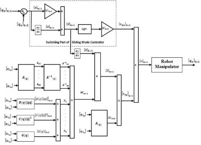
Fig. 4. Block diagram of PD sliding mode controller for robot manipulator

According to the literature stability is very important and influential case to select and test a controller and conventional sliding mode controller based on discontinuous controller part is a stable controller. Consequently proof of stability based on the Lyapunov function is determined by the following equations. The lyapunov formulation can be written as follows,

• У = -$Г.А$

and the derivation of V can be determined as,

• У = 1sr.AS + Sr AS

the dynamic equation of robot manipulator can be written based on the sliding surface as

AS = -PS + AS + B + C + G

Since A — 2V is skew-symetric matrix, therefore it is written by;

. 1_ .

SrAS + - ST AS = Sr(AS + PS)

If the dynamic formulation of robot manipulator defined by	Ku ≥|[ ̃ ̇+ VS + G ]|+ q,              (123)
Т=( q ) ̈+ V ( q , ̇) ̇+ G ( q )                (112)	Resulting, the following formulation guaranties the stability of the Lyapunov equation in sliding mode
the controller formulation is defined by	controller with switching (sign) function.
T= ̂ ̈ + ̂ ̇ + ̂+ К sgn ( S )            (113)	̇≤-∑ q, | st |                          (124)

According to (112) and (113), can be expressed:

A(q) ̈+v(q, ̇) ̇+G(q)= ̂ ̈ + ̂ ̇ + ̂+К sgn(S )                     (114) Boundary layer chattering free method: According to the literature to attenuate the chattering challenge, linear boundary layer method based on saturation function is introduced. In this method the researcher introduced Since ̇  = ̇ - and ̈  = ̈- ̇ saturation function in the sliding mode control law instead of the switching (sign) function in (102). The Ȧ+(V+A)s=∆f-к               (115) saturation (linear) method with small neighborhood of the switching surface is calculated as [6]. the dynamic equation of robot manipulator can be written based on the sliding surface as В(t)={X,|s(t)|≤∅};∅>0            (125) Л̇=-vs +Л̇+vs +G-T            (116) where ∅ is the boundary layer thickness. Consequently the sliding mode function in (102) can be written by; Assuming that it can be expressed by the following equation: и=  (⃗⃗, t)∙Sat .5⁄∅/                     (126) ST( ̇-2V)s=                         (117) While saturation function formulation (Sat . 5 ⁄ / ) is as follows [1] and with regard to substituting (117) in (110); ̇=|ST ̇ IS - STVS + ST (Ȧ+VS +       (118) G-T)=ST (Ȧ+VS +G-T )            (118) ⎧ 1        ( 5 ⁄∅>1) sat .5⁄∅/= -1        .S⁄∅<-1/     (127) ⎩⎪ 5 ⁄∅    (- 1 ̂= ̂ +7̂s=[t̂1( ̂+ ̂)+ ̇] ̂      (119) +К․ sgn (s              (119) Considering the above points, to reduce chattering phenomenon in sliding mode controller based on saturation function, the following formulation is used [16]: by replacing the equation (119) in (118) т=    + ^-sat                                (128) ̇=ST (Ȧ+VS +G-̂ ̇- ̂S- ̂- Ksgn (s)=ST.̃ ̇+ ̃S+ ̃-          (120) Ksgn (s)/ and T  can be calculate as follows: ^eq =[A"1 (В+C+G)+ ̇]A             (129) and it is clear that |̃ ̇+ ̃S+ ̃|≤|̃ ̇|+| ̃S|+| ̃|        (121) To reduce or eliminate the chattering linear (saturation) boundary layer method used by many researchers. However eliminating the switcℎing discountinous the Lemma equation in robot manipulator system is function in sliding mode controllers are used in many research but it can causes to lost the robustness of control Ku=[| ̃ ̇|+|VS|+|G|+q] ,= 1,2,3, ,…                       ,                (122) and accuracy. Fuzzy Controller Operation: A robot manipulator consider as a nonlinear and MIMO system with outputs the equation (117) caused; available measurement and possibility to input change. According to design sliding mode controller, this controller can be used as a controller when it has a satisfying result and system is easy to implement but if some information about robot manipulator operation or controller is available and it can be formulated as a set of rules and fuzzy controller is used to control of robot manipulator. However the application of fuzzy logic controller is really wide, all types of fuzzy logic controllers consists of the following parts;

• •    Choosing inputs

• •    Scaling inputs

• •    Input fuzzification (binary-to-fuzzy[B/F]conversion)

• •    Fuzzy rule base (knowledge base)

• •    Inference engine

• •    Output          defuzzification          (fuzzy-to-

• binary[F/B]conversion)

• •    Scaling output

Figure 5 shows the block diagram of fuzzy controller operation.

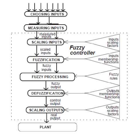
Fig. 5. Block diagram of Fuzzy Controller Operation [30]

Define the inputs and control variables: based on controllers’ design select the type of inputs is very important to design controller. In most of industrial controllers error and the functional of error are used as inputs to design controller. According to design the linear controller, PI, PD and PID are three types of linear controller. If PI like fuzzy controller is design, error and integral of error are introduced as fuzzy input. In PD like fuzzy controller error and change of error are used to define as controllers’ inputs. According to design PID controller, PID like fuzzy controller has three inputs; error, change of error and integral of error. To design fuzzy controller, if one has made a choice of designing a type of PD like fuzzy controller, PI like fuzzy controller or PID like fuzzy controller, this already dealing the choice of process state and control output variables, as well as the content of the antecedent and consequent parts for each rule.

Scaling inputs/outputs: in fuzzy logic controller to define membership function, first of all one needs to consider the universe of discourse for all inputs and outputs linguistic variables. If universe of discourse indicates by small range of scaling input or output, the data can be off the scaling. Conversely, if universe of discourse indicates by large range of input scaling, the membership function area can be wide on the left or right side if scaling input or output. The role of a right choice of scaling factors is obviously shown by the fact that if your choice is bad, the actual operating area of the inputs/outputs will be transformed into a saturation or narrow situation. Input scaling factors have played important role to basic sensitivity of the controller with respect to the optimal choice of the operating areas of the input signals. When the scale output is scaled, the gain updating factor of the controller is scaled. This item affects the closed loop gain and caused to modify the stability and oscillation tendency. Because of its strong impact on stability and reduce the oscillation, this factor is important factor to design fuzzy controller. The right choice of input/output scaling factor shows in Figure 6.

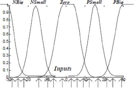
Fig. 6. Right Choice of the Scaling factor [30]

Input fuzzification (binary-to-fuzzy [B/F] conversion): fuzzification is used to change the crisp set into fuzzy set. This part is divided into three main parts;

• •    Linguistic variables

• •    Scaling factor (normalization factor)

• •    Inputs membership function

A linguistic variable is a natural language based on the quantity of interest. These variables are words or sentence and this is the main difference between linguistic variable and numerical variable. Linguistic variables can be divided into three sub parts:

• •    Primary terms, which are the labels of location of the universe         of         discourse         (e.g.

Negative or Positive or Zero).

• •    Connective terms AND, OR, and NOT.

• •    Limitation terms such as Small, Medium and Big.

A linguistic variable is defined by;

• •    Symbolic name of inputs/outputs variables such as error,cℎange of error and Torque .

• •    Set of linguistic values that can take on some variables such as, Negative Big (NB), Negative Medium (NM), Negative Small (NS), Zero (Z), Positive Small (PS), Positive Medium (PM), Positive Big (PB).

• •    Scaling factor as actual physical domain over which the meaning of the linguistic value, for example and based on literature [33] and experience knowledge if error is between -1 and +1.

• •    Interpretation of linguistic value in terms of the quantities values.

Select the membership function has a below challenges;

• •    Select the general parameters , such as the number of membership functions to support all the values of the linguistic variable on the universe of discourse

• •    The location of membership functions on the universe of discourse

• •    Width of the membership functions

• •    Continous parameters, such as the shape of a particular membership function

Figure 7 shows the fuzzification part for PD like fuzzy controller system, this PD like fuzzy controller has two inputs (error and change of error), any input is described with five linguistic values; Negative Big (NB), Negative Small (NS), Zero (Z), Positive Small (PS), Positive Big (PB), they are quantized into four levels between -2 and +2, and triangular membership functions are used for error and change of error inputs.

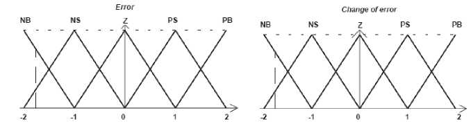
Fig. 7. Fuzzification part fuzzy controller [30]

Fuzzy rule Formulation: the role of the rules in fuzzy logic controller is extremely significant and the main approaches and source of fuzzy logic controller rules are;

• •    Expert experience and knowledge base

• •    Learning based on operators’ control action

• •    Identification of fuzzy model system under control action

• •    The application of learning technique

According to above, the main approach comes from an expert knowledge of system because any fuzzy controller is expert system to solve the control problem. Based on linguistic variables, fuzzy rule base provides a natural theory for human thinking and knowledge base formulation. In practice to find the rule base two method are introduced;

• •    Design rule base based on redeveloping literature, manuals and research papers

• •    Design and develop of rule base based on the inquiry operator using questionnaire.

In practice fuzzy rule base divided into main three parts: antecedent part, consequent part and connective terms (AND, OR, NOT). The OR term of two fuzzy set e and ṫ is a new fuzzy set which the new membership function is given by

∀ It ∈U

The AND term of two fuzzy set e and ̇ ( T- norm) is a new fuzzy set which the new membership function is given by

In fuzzy set and the NOT e operation can be replaced by 1-e operation in fuzzy set.

Frequently the rules are formulated one by one base on experience knowledge and any other methods and rule table is design after complete all rule bases. Rule table is the dynamic behavior of fuzzy logic theory and it necessity to have three significant parts;

• •    Continuous

• •    Complete

• •    Consistent

If two fuzzy rule base formulated as follow;

F․ R1:                   ̇ is NB tℎen T is PB

F․ R2 :                    ̇ is PS tℎen T is Z

Inference Engine (Fuzzy rule processing): The fuzzy inference engine recommends a fuzzy method to transfer the fuzzy rule base to fuzzy set. Fuzzy rule processing is divided into two main techniques;

• •    Mamdani method

• •    Sugeno method

Mamdani anticipated controlling the system by realizing various fuzzy rule bases. In Mamdani controllers’ design, in order to improve the control quality, he increased the number of control inputs and used the change of variable error in his design. He designed his controller on the PDP-8 computer. It contained 24 fuzzy rule bases. According to his experiments, the quality of the fuzzy controller based on the 24 fuzzy rules was found to be better than the best result of the fixed conventional controller, as a result fuzzy controller opening a new epoch in a design controller. This type of fuzzy inference is easily understandable by human experts, simple to formulate rules and proposed earlier and commonly used.

Michio Sugeno is changed a part of the rules, in consequent part of fuzzy rule base. According to this method, the consequent part is a mathematical function of the input variables. This type of fuzzy inference is more efficient computationally, more suitable in mathematical analysis, and guarantee the output continuity surface. The following definition shows the Mamdani and Sugeno fuzzy rule base

Mamdani    F․ R¹:

then T is PB

Sugeno       F․ R¹ :

then 0․3×e+0․6× ̇ is PB and ̇ is NB and ̇ is NB    (132)

In these two types inference engine the antecedent part are the same but the main difference between these two methods are in consequent part. Fuzzy inference system has two main parts;

• •    Rule evaluation

• •    Aggregation degree

Rule evaluation is used to illustrate the fuzzy operation (AND /OR ) impact to the antecedent part of the fuzzy rules.

The aggregation degree is the aggregate two neighbouring fuzzy rules and makes a new consequent part. It is note that activation degree is the impact of antecedent part to consequent part and aggregation degree is the impacts of the first modify consequent part in the second one. Several methodologies are used to calculate aggregation degree;

• •    Max-Min aggregation

• •    Sum-Min aggregation

• •    Max-bounded product

• •    Max-drastic product

• •    Max-bounded sum

• •    Max-algebraic sum

• •    Min-max aggregation

The formulation of Max-min aggregation is

The formulation of Sum-min aggregation is;

Defuzzification: defuzzification is the last step to design fuzzy logic controller and it is used to transform fuzzy set to crisp set. Consequently defuzzification’s input is the aggregate output and the defuzzification’s output is a crisp number. Two main techniques to calculate the defuzzifications are;

• •    Centre of gravity method (COG)

• •    Centre of area method (COA)

The formulation of COG method is;

COG(x_k, Ук)

The formulation of COA method is

COA (x_k, Ук )

Based on above formulation, COG(Xr, Ук ) and COA (Xr,У к ) illustrates the crisp value of defuzzification output, ∈и is discrete element of an output of the fuzzy set, Ци․(Xk ,У к, ) is the fuzzy set membership function, and г is the number of fuzzy rules.

• III.    Methodology

Serial links, six degrees of freedom PUMA robot manipulator has highly nonlinear dynamic equations, MIMO, time variant dynamic equations, uncertain and there exist strong coupling effects between joints, consequently, minimum couple effects, stable, robust and reliable controller obligation used to control of this system. The problem of coupling effects can be reduced, with the following four methods:

• •    Limiting the performance of the system according to the required velocities and accelerations, but now the applications demand for faster and lighter robot manipulators.

• •    Using a high gear ratio (e.g., 250 to 1) at the mechanical design step, in this method the price paid is increased due to the gears.

• •    Linearization and decoupling without using many gears based on feedback linearization methodology by measurement actual acceleration.

• •    Proposed methodology

In linear control methodology to reduce the coupling effect limiting the performance and high gear ratio is recommended, which caused to have an expensive and slow robot manipulator. To reduce the coupling effects based on computed torque controller two challenges are emerge; need to have the accurate dynamic model which it is very difficult and measurement the actual acceleration that it is very expensive. To reduce the coupling effect based on proposed methodology all above challenges can be eliminate. In proposed methodology select the desired sliding surface and sign function play a vital role and if the dynamic of robot manipulator is derived to sliding surface then the linearization and decoupling through the use of feedback, not gears, can be realized. In this state, the derivative of sliding surface can help to decoupled and linearized closed-loop PUMA robot dynamics that one expects in computed torque control. Linearization and decoupling by the above method can be obtained in spite of the quality of the robot manipulator dynamic model, in contrast to the computed-torque control that requires the exact dynamic model of a system. As a result, uncertainties are estimated by discontinuous feedback control and the linear part controller is added to this part to eliminate the chattering. Linear controller is type of stable controller as well as conventional sliding mode controller. In proposed methodology PD, PI or PID linear controller is used in parallel to discontinuous part to reduce the role of sliding surface slope as a main coefficient. Based on Lyapunov methodology, proposed method is highly robust and stable controller. In PD controller the control law is given by the following equation;

Where е   ^Qid^{+ Q}ia and е = Q ' id + Q ¹ i_a .

In this theory Kp and Kvi are positive constant. To show this controller is stable and achieves zero steady state error, the Lyapunov function is introduced;

1

• V = 2 [q ^T A(q^)q + e^T K_pe]

• ¹d²T                                    (138)

• 2 at

Where Q T is the power input from actuator and 2^d [Q '^T AQ] is the derivative of the robot kinematic energy.

V = qT[Т+ Kpe](139)

Based on T=-K_p^e - Ky^е , we can write:

V = qT Kpq̇ ≤0(140)

If V = 0 , we have q = 0 ^ q = 0 ^ q = A-1Kpe →e=0(141)

In this state, the actual trajectories converge to the desired state.

In proposed method

n

V=<1^i | Si | i=i

In this method:

S= S(e,ė)= Ae +ė=0 ,    A>0

Ṡ=Aṫ+ /(e,e ̇, t)+U,S (0) = So

In this case;

Udis = k sgu(S)=k sgu(Xe +t ̇), X> 0 ,k>0

According to linear methodology;

Ulin   Kp^e + Kvie ̇,

Kp. > 0 , K^t>0

And if K_vi = 1 then

^Ulin   ^Kp^^{e +}ė=^Si                           (148)

Uproposed = Udis + Ulin = k sgu(Xe +ė)+ Ulin

According to above, proposed method is stable and it also can chatter attenuation using linear sliding surface method.

The second objective in this paper is reducing the sensitivity to system’s dynamic formulation. To solve this challenge PD plus integral fuzzy logic theory is used in this research. To compensate dynamic formulation of robot manipulator Mamdani fuzzy inference system is introduced. To achieve this goal, the mathematical dynamic formulation of pure sliding mode controller is modeled by Mamdani’s fuzzy logic methodology. Fuzzy logic method has the following specifications: two inputs (error and the rate of errors); an output (Torque); 7 linguistic variables for any inputs and outputs (Negative Big, Nagative Medium, Negative Small, Zero, Positive Small, Positive Medium, Positive Big), therefore it has 49 rule bases for any link; and triangular membership function also is used. However PD fuzzy logic theory is used but the integral part is used to estimate the steady state error. Figure 8 shows PD fuzzy plus integral sliding mode controller.

Based on Figure 8, the fuzzy compensator sliding mode controller’s output is written;

11

V= ST AS + - [q T Aq + eT Kpe]

̂ aYN puz^y + ^modified-SMC

and the derivative of V is;

and ^d^yn puzzy is calculated by;

1

^DYNfuzzy =∑iheT^(X)  +  [A-1 (Q)×

(N(Q, q)) + S] x A(Q)

then

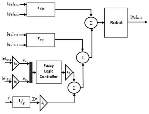
Fig. 8. Block diagram of PD+I modified fuzzy sliding mode controller

• IV.    Results And Discussion

To test of this methodology conventional sliding mode controller and proposed methodology are compared. Chattering elimination, trajectory tracking and disturbance elimination are quality reference in this test.

Chattering elimination: linear band controller in conventional sliding mode controller provide a perfect chattering elimination for a reference trajectory with a negligible tracking error in Figure 9.

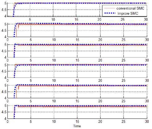
Fig. 9. Linear band SMC and Conventional SMC

According to Fig 9; conventional sliding mode controller has chattering in all 6 joints but chattering can be eliminate by linear band sliding mode controller.

Tracking Control of Proposed Method: trajectory followings of 6 DOF for conventional sliding mode and proposed methods are compared in Fig 10. According to the simulation result, traditional sliding mode controller has high frequency oscillation chattering. To chattering attenuation PD+I fuzzy linear band sliding mode controller is introduced. According to Fig 10, conventional sliding mode controller is faster than proposed method.

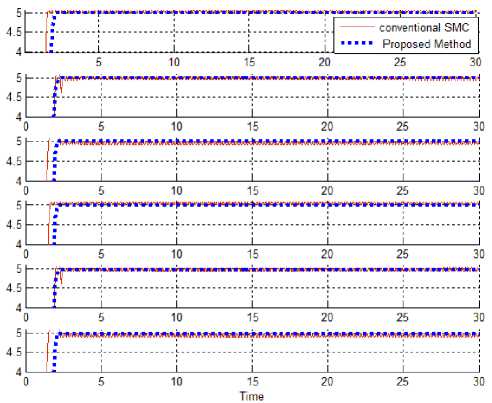
Fig. 10. Conventional SMC and Proposed method

Comparison the disturbance rejection: the power of disturbance rejection is very important to robust checking in any controllers. In this section trajectory accuracy is test under uncertainty condition. To test the disturbance rejection band limited white noise with 30% amplitude is applied to conventional sliding mode controller and proposed controller. In Fig 11, trajectory accuracy is shown.

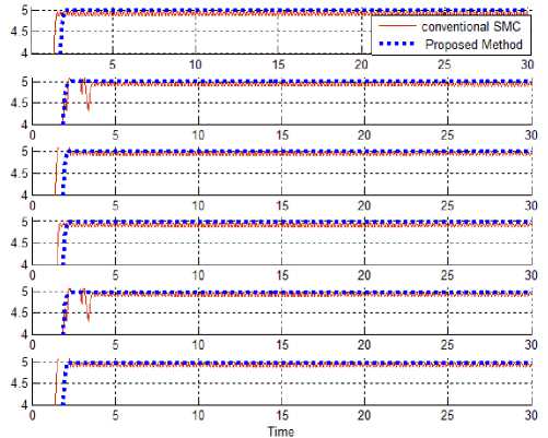
Fig. 11. Comparison of disturbance rejection: Conventional SMC and Proposed Method in presence of uncertainty

• V.    Conclusion

The work conducted in this paper has been multidisciplinary and wide in scope ranging from the design of a multi-axis robot manipulator to understanding of non-linear control and artificial intelligence. At the outset of the research paper, this research aimed to introduce intelligent improve nonlinear controller to highly nonlinear manipulator structures. With the topical research work on conventional sliding mode and fuzzy logic theory, this project was further motivated by the need to investigate the design and improve of new type robust chatter-free sliding mode controller. This research follows two main targets: reduce the chattering phenomenon based on conventional theory in presence of switching part methodology and estimate the nonlinear dynamic equivalent part of system according to the design (PD+I) MAMDANI fuzzy theory. The main benefits in this is eliminate the chattering as well as robust in uncertain condition based on linear band sliding mode controller and fuzzy logic theory. The research result (Figures 10-11) illustrates that proposed method can guarantee stability and robustness.

Acknowledgment

The authors would like to thank the anonymous reviewers for their careful reading of this paper and for their helpful comments. This work was supported by the Department of Electrical Engineering University Putra Malaysia.