Detection of anomalies in fetus using convolution neural network

Published Online November 2018 in MECS DOI: 10.5815/ijitcs.2018.11.08

Abnormality in Fetal development has become a bane to the society. The detection rates of these fetal abnormalities are low till date. Ultrasound is one of the tool used for determining the health of a fetus. Doctors prefer ultrasound due to low cost, wide availability, real-time capabilities and the absence of harmful radiation. But the accuracy of ultrasound imaging is limited due to poor signal-to-noise ratio, poor penetration through bone or air and also air or bowel gas prevents visualization of structures. In addition to that the fetus may not have a favorable position in the womb to get a clear image of the required part.

Presently, ultrasound scan during the mid-pregnancy period i.e., between 18-22 weeks has been a required and recommended routine during the gestation weeks. It reveals the size of the baby after 6 weeks [9]. These scans also shows the position where the baby is lying, bio statistic measurements are noted (e.g. head circumference on the trans-ventricular head view) and possible abnormalities are detected in the later development stages.

Directing the ultrasound scan probe to the correct scan plane can be a sophisticated task and also much depend on the qualifications, skill and experience of the ultra-sonographer, as well as their ability at interpreting the images. Even experienced and adroit ultra-sonographers with the best equipment can give false positives or false negatives. As a result, there is a significant sufferings from low reproducibility and large operator bias [1]. Screening deals with capturing the correct image which in turn needs years of experience which cannot be carried by an amateur. In addition to that there is also significant scarcity for skilled sonographers. The International Clearinghouse for Birth Defects Surveillance and Research is a voluntary non-profit international organization in official relations with WHO which brings together fetal anomalies surveillance and research programmes around the world.

In order to investigate and prevent congenital anomalies and to lessen the impact of their consequences, we propose a medical decision support system based on CNN for real time automated and reliable detection of fetal anomalies which requires immediate parental care, like Spina bifida, anencephaly, microcephaly, thick abdominal wall. We have modelled the system for all of the standard cases that occur during the pregnancy for all the fetal anomalies mentioned, plus the most commonly acquired fetal views. The localization can be achieved during training with only screening level image labels available through scan planes. This is an important task in the model developed because bounding box annotations are not a regular pattern documented and would also be time consuming for larger datasets. Our approach achieves real-time performance, time efficiency and high accuracy in the detection task based on the localization on the ultrasound images. All analysis is conducted on ultrasound image data which is obtained during full mid-pregnancy examinations since it is the viable time for getting clear images of the fetus.

The proposed system can be used in many productive ways. It can be employed to provide real-time feedback about the ultrasound image to the sonographer. This may decrease the number of misinterpretations made by any inexperienced sonographer. Since the model gives quick results it saves time during an emergency situation. The localization of target shapes in the images has the potential to help non-experts in the detection and diagnosis of tasks in a much easier and efficient way. This may be particularly useful for training purposes for the applications in the developing world. Hence we hope to build trust into the method presented and also to guide instinctively to understand failure cases.

Automated detection and localization of standard fetal anomalies are the core pre-processing steps for other automated image processing.

• II.    Literature Review

Few papers have proposed various methods to detect fetal anomaly using ultrasound images, ECG (e.g. [4, 7 and 8]). The authors here have concentrated on detecting a specific fetal anomaly such as heart defects or abdominal defects rather than the general standardized fetal anomalies. A very few papers have proposed different methods on Detection Fetal Standard Scan planes in Freehand Ultrasound [6] but not many works have been done in the field of general standard fetal anomalies.

Gustavo Carneiro et. al presented a system that automatically measures the BPD and HC from ultrasound images of fetal head, AC from images of fetal abdomen, FL in images of fetal femur, HL in images of fetal humerus, and CRL from images of fetal body [1]. This system utilizes a huge database of annotated images in order to model statistically the appearance of such structures. This is achieved through the training of a Constrained Probabilistic Boosting Tree classifier. In this model there is a need of all measurements of the fetus which in turn requires a lot of memory and processing time for the detection.

The fuzzy logic method used to observe the movement of the fetus once the video frames are pre-processed is conveyed in [2]. The system gives information about any movement of the fetus stage by stage and also its development is observed.

Fetal Cardiac Heart Defects such as heart rate detection, valve defects etc., detected using ECG, Doppler Cardiogram Signals, and Doppler Ultrasound Signals are conveyed in [3, 4, 5, and 7]. These works relay on the approaches like Image Classification [8], recurrence qualification analysis [5], feature extraction etc. The authors in the above works have concentrated on only specific fetal anomalies like heart defects. There are not many work published on a reliable medical decision support system for standard fetal anomalies the also need immediate care.

Our paper is most closely related to Christian F. Baumgartner [6]. It presents a novel method using CNN to detect the standard scan planes of the fetus on freehand ultrasound. Here the pre-processing is carried in 5 main steps. This pre-processing is efficiently reduced to 3 main steps in our work. A significant difference between the present study and above works is that the latter work is only to a precise fetal defect like CHD (functional defects). However, it is not the case that fetuses can only have heart defects. Hence there is a need for a reliable medical decision support system that can detect the fetal anomalies that are as severe as CHD. The above works which have ultrasound data usually use 4 main steps for detection i.e., noise removal, segmentation, feature extraction, classification. This results in a tedious work since it requires a lot of processing time and memory for every step. This complexity is eliminated in the presented work by using CNN, which handles all the above preprocessing steps in an efficient manner.

Localization using CNN is an active field of research in Image Processing [6]. Here an attempt is made in this direction to determine fetal anomalies using ultrasound image data.

• III.    Methodology

• A.    Dataset

Our dataset consists of ultrasound image evaluations of the fetus during the mid-pregnancy gestational ages between 18–22 weeks which have been acquired during routine screenings by expert sonographers. The dataset contains of fetal normal images along with the abnormal cases.

• B.    System Design

The system design flow is instigated by input image acquisition. Here an ultrasound image from the dataset is given as input for testing.

Pre-Processing being the next step of design is carried in 3 steps as shown in the Fig.1

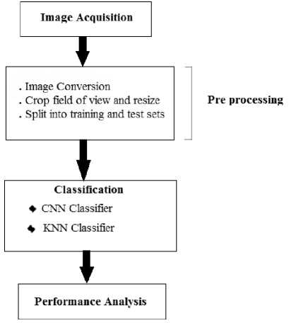
Fig.1 Design Flow of the system

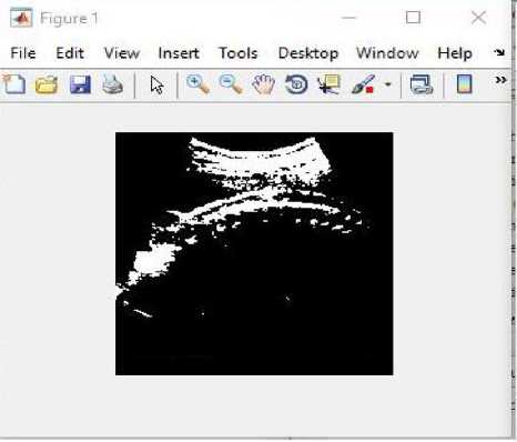
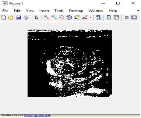
In order to remove all the freeze-frame images and also to make the pre-processing easier and quicker, image conversion is done. Here the given input image is converted into a binary image.

All image and frame data are resized and cropped to a 224×288 region containing the good field of view. We resize an image so that the pixel size of an image is altered, then the image is resampled to create a new set of pixels compatible to the new pixel size. If we reduce the image, several pixels or parts of pixels in the former image will add to one pixel in the new image. This means that we will lose details of the image. However, we are likely resizing the image to use it at that reduced size, so that we will not see the loss of detail. After resigning the image, the same will be converted into Binary image for further processing. The Binary image is illustrated as in Fig.2.

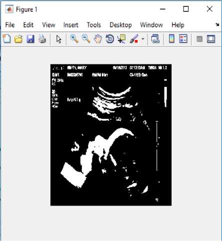
Fig.2. Converted binary image

Ultrasound image data contained lesser number frames of the fetus than the background frames. Hence, it was possible to create a background class by randomly sampling frames from the ultrasound image. In order to decrease these random sampling of the image frames, frames were only sampled in the fetus region of the image. In the last stage, we split all of the cases into training set containing 80% of the cases and test set containing remaining 20%. The split was made on the case level rather than the image level to guarantee that no image originating from the test images were used for training.

Classification is an important stage in identifying type of the defect present in the input scanned image of the fetus. The features selected for the anomalies are: 1) shape of the fetus in the region of interest 2) patterns of the image where anomalies are present. In classification classifier is used for object recognition and classification. The classifiers recognize the object and classify based on the extracted features of an image given as an input. This is achieved with the help of CNN associated with KNN.

• C.    Network Architecture

The proposed work is a layered model, which consists of 3 layers: input layer, intermediate layer and output layer. CNN is applied to image data in the input layer. Depending upon bit size, the pixel value matrix and the array of value can be programmed easily. A single pixel can be represented as [0,255]. However, RGB consists of separate color channels which makes the input image as 3D.Thus the input image consists of three color channel matrices.

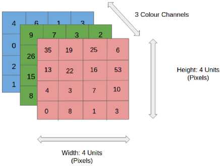
Fig.3. Input image consisting of three color channel matrices

Output Layer is where the given image is predicted as either normal or one of the following anomalies: Anencephaly, Microcephaly, Spina bifida and Thick abdominal wall. The output image depicts where exactly the anomaly is present on the output image.

Convolution Neural Network is mainly conceptualized in the intermediate layer. It consists of convolutional, subsampling and fully connected layers. The First layer of a convolutional neural network with pooling is as shown in Fig.4.

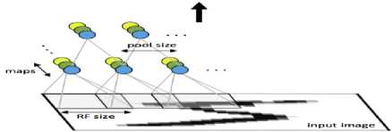
Fig.4. First layer of a convolutional neural network with pooling.

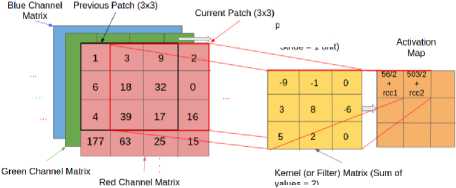
During the convolution of a Kernel with the given input volume works by taking patches from the input image whose size is equal to the kernel size and values are convolved between the values in the patch and the kernel matrix. By summing the resultant terms single entry is made in the activation matrix [10].

The convolved value is obtained by summing the resultant terms from the dot product forms a single entry in the activation matrix. The patch selection is then slided by a certain amount called the ‘stride’ value, and the process is repeated until the entire input image has been processed [10]. The process is demonstrated in the Fig.5.

(Obtained after sliding from previous position by 1 unit, i.e. Stride = 1 unit)

values = 2)

Fig.5. The convolution value is calculated by taking the dot product of the corresponding values in the Kernel and the channel matrices.

The current path is indicated by the red-colored, bold outline in the Input Image volume. Here, the entry in the activation matrix is calculated as:

AM[1][2] = Red Channel Matrix Contribution(CMC)+Green CMC+ Blue CMC = [(3,9,2).(-9,-1,0) + (18,32,0).(3,8,-6) +

(39,17,16).(5,2,0)]/2 (From-red-channel) + rcc2 = [-27-9+0+54+256-0+195+34+0]/2 +rcc2

= 503/2 +rcc2                  (1)

where rcc2 refers to the contribution from the remainder channels.

Given an input volume, connecting all neurons with this may lead to many weights to be trained as a result it produces high computational complexity. Instead of this we specify a 2 dimensional region called ‘receptive field’ with encompassed pixels connected to neural networks input layer [10]. Each layer of CNN has specific task of transforming its input into a useful representation. CNN architecture in this study is specifically concentrated into 3 major layers. The processing that an input image goes through these layers is discussed below. Conv Layer is another name of Convolution Layer which forms the basis of CNN and performs training operations in order to fire the neurons of the network as shown in Fig.6.

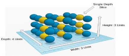
Fig.6. Convolutional layer representation in 3D

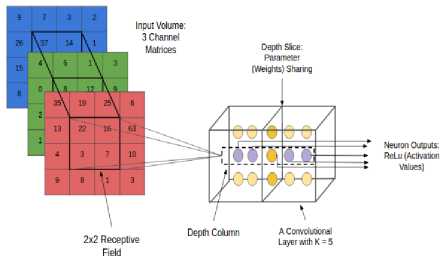
Fig.7. Receptive Field.

The ReLu Layer then calculates the non-linear property of the image. ReLu (Rectifier Unit) is one of the most commonly applied activation function for the outputs of CNN neurons [10].

The Next layer after the Convolutional layer is pooling layer. It performs ‘down-sampling’, which deals with reduction of size which in turn leads to loss of information. Due to this loss of information there are several benefits to the network: 1) Size reduction leads computational overhead for the upcoming layers of the network becomes less 2) It works against over-fitting.

The pooling layer takes a sliding window or a certain region that is moved in stride across the input transforming the values into representative values. The transformation is either performed by taking the maximum value from the values observable in the window or by taking the average of the values. Then for each color channel, the values will be down-sampled to their representative maximum value if we perform the max pooling operation as in Fig.8. By this operation no new parameters are introduced in the matrix.

An input image under goes repeated loops of the above three layers until it is stable for the detection operation to be operated on it then it is passed on to Fully Connected layer where the image is configured it is fully connected with the output of the previous layer[10].

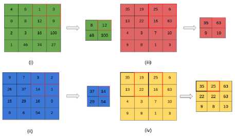
Fig.8. The Max-Pooling operation can be observed in sub-figures (i), (ii) and (iii) that max-pools the 3 color channels Sub-figure (iv) shows the operation applied for a stride value of [1, 1], resulting in a 3×3 matrix

The motivation behind using CNN is to predetermine the node weight of the region of interest during training and to compare these node or neuron values with the input image given during testing. This comparison is done using one of the most efficient algorithm i.e., K-nearest neighbour algorithm. KNN compares the node weight of given input image to the nearest predetermined node weight of the images in the training dataset to determine the anomaly present in the image.

A simple case to depict the working of KNN is shown in Fig.9 and Fig.10. The figure consists of random red circles (RC) and green squares (GS) as shown in Fig.10.

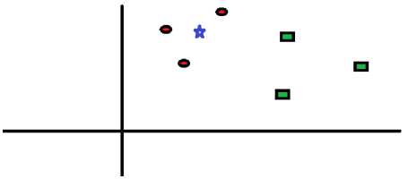
Fig.9. Data points in the plane

If one wants to find the class of Blue Star (BS). The “K” in KNN algorithm is the nearest neighbours is applied. Let us say K = 3, then we will make a big circle enclosing three RC as depicted in Figure.11. All three data points (RC’s) are closest to BS(Blue Star).Hence we can say that BS should belong to RC. Selection of parameter K plays a very crucial role.

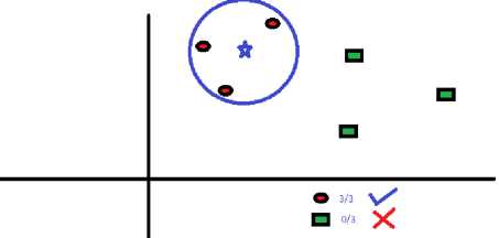
Fig.10. Enclosing data points on the plane

Following Fig.11 are the different boundaries separating the two classes with different values of K.

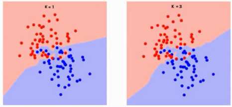
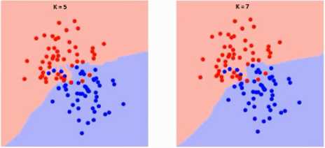
Fig.11. Different boundaries separating the two classes with different values of K.

With the increasing value of K the boundary becomes smoother as shown in Fig.11, When K reaches infinity it becomes all blue or all red.

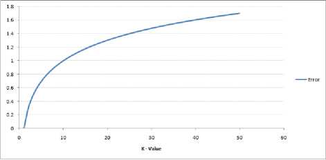
Fig.12. Curve for the training error rate with varying value of K

The error rate at K=1 is always zero for the training sample as shown in Fig.12, because the closest point to any training data point is itself. Fig.13 shows the validation error curve with varying value of K:

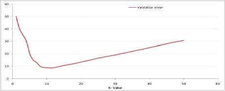
Fig.13. Validation error curve with varying value of K.

Implementation of KNN Model:

• 1)    Load the data.

• 2)    Initialize the value of k.

• 3)    From 1 to total number of training data points are iterated and predicted class is obtained.

• •    Based on Euclidean distance, the distance between test data and each row in training data is calculated and these calculated distances are sorted in ascending order.

• •    From the sorted array [13] top k rows are selected and among this most frequent class is selected.

• •    Return the predicted class.

• D. Training

In Computer Vision systems, datasets are divided into two main categories: a training dataset used for training the algorithm learn to perform its desired task and a testing dataset that the algorithm is tested on. The percentages that one divides them by affects the general pipeline and it is the first step when trying to solve this challenging task. The work that is being offered within this paper, focuses on an 80% - 20% split across all datasets. Furthermore, each training and testing dataset is further split into negative and positive structures in order to make sure that the algorithm learns what it should be looking for in an image as well as what not to look for. At the end of a test run, one needs to look at all accuracy counts to be able to come up with a total analysis of the pipeline created.      This need emphasizes the fact that the system learns how to better optimize itself. Using previous research work as a base, a comparison of several types of CNN architectures is made. To have as conclusive results a complex and full analysis as well as making sure that the learning process is beneficial for the entire pipeline, and particularly for the feature extractors, four widely used main datasets have been selected for training and testing purposes.

In image processing, training and testing is an instance used for categorizing pixels in order to section different objects. A common example is to use a random forest classifier: the user selects pixels belonging to the different objects of interest (eg background and object), the classifier is trained on this set of pixels, and then the remainder of the pixels are credited to one of the classes by the classifier. The training cases are: 1. Normal fetal images 2. Abnormal fetal images like Anencephaly, Microcephaly, Spina Bifida, and Thick Abdominal Wall. The major steps in training a dataset if ‘m’ is the number of training data samples and p is an unknown point are:

• 1)    Store the training samples in an array of data points arr[]. This means each element of this array represents a tuple (x, y) [14].

• 2)    for i=0 to m:

• 3)    Calculate Euclidean distance d(arr[i], p).

• 4)    Make set S of K smallest distances obtained. Each of these distances correspond to an already classified data point.

• 5)    Return the majority label among S.

• IV.    Experimental Results and Discussions

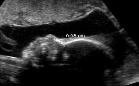
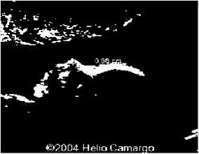
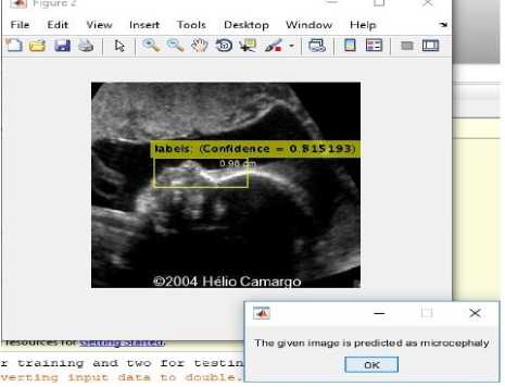
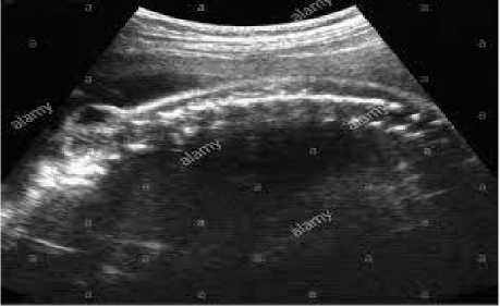
After the collection of fetal ultrasound images in all most all the cases mentioned in the paper, the accurate results are predicted with respect to any fetal position inside the mother’s womb. Tests for the detection accuracy using the ultrasound image data mainly consists of training of the dataset. Accumulation of the dataset had also been one of the most crucial task in this paper since it is not the case that all the fetuses will have abnormalities. The algorithm in this paper is trained in such a way that it can detect any of the anomalies mentioned above even if the fetus is at any position in the womb. This accuracy or confidence level of the whole project ranges around 85%. The accuracy can be increased by increasing the training dataset given for training. After the input image is given it is converted into a binary image then a image appears which consists of bound box on it screening where exactly the anomaly is present. Finally an annotation appears depicting the fetus anomaly. This screening for all the cases discussed in the paper are shown in figures below.

(i)

1*1 Figure 1                                     —     □ X

File Edit View Insert Tools Desktop Window Help           "^

■2i a ^ ^ b x x o® € ^-ia no □ □

(ii)

(iii)

Fig.14. (i) Input image for testing (ii) Converted binary image of input image (iii) Anomaly predicted as microcephaly as shown in dialog box.

(i)

(ii)

(iii)

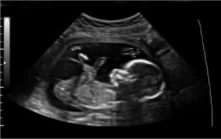
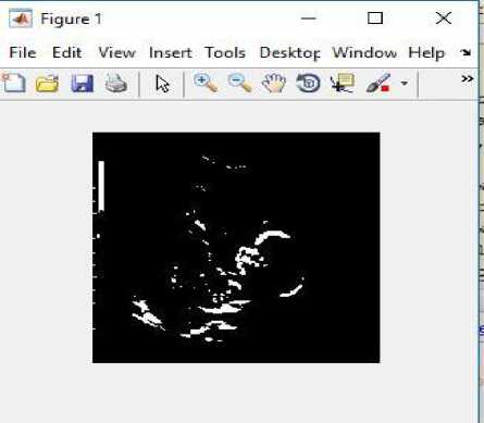
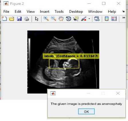
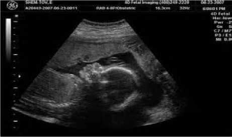
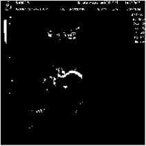
Fig.15. (i) Input image for testing (ii) Converted binary image of input image (iii) Anomaly predicted as anencephaly as shown in dialog box.

(i)

(ii)

(iii)

(iii)

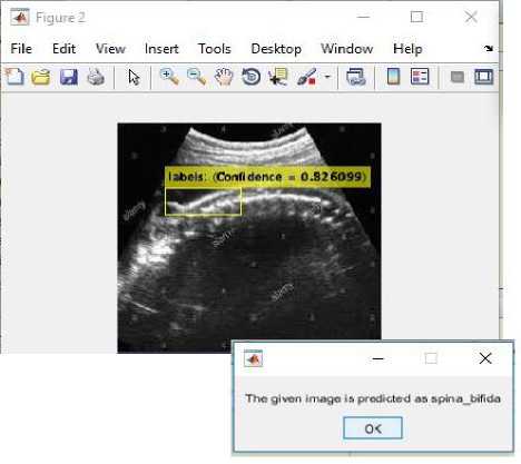
Fig.16. (i) Input image for testing (ii) Converted binary image of input image (iii) Anomaly predicted as spina bifida as shown in dialog box.

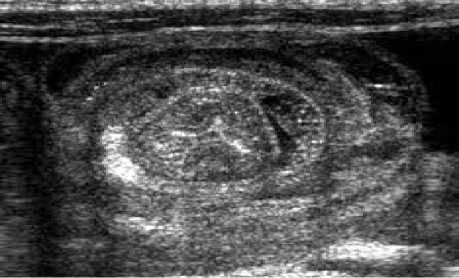
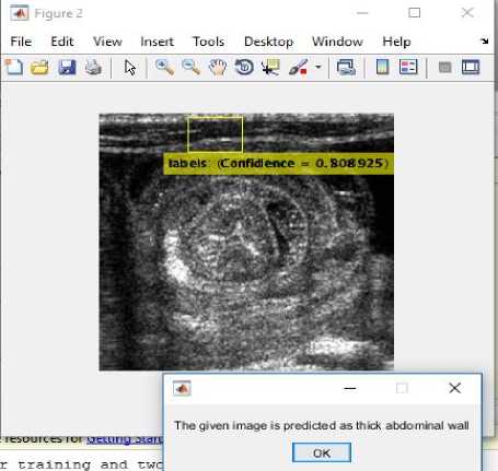
Fig.17. (i) Input image for testing (ii) Converted binary image of input image (iii) Anomaly predicted as thick abdominal wall as shown in dialog box.

(i)

Л Figure 1                              —    □ X

(i)

(ii)

File Edit View Insert Tools Desktop Window Help ^

(ii)

(iii)

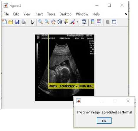
Fig.18. (i) Input image for testing (ii) Converted binary image of input image (iii) Fetus predicted normal as shown in dialog box.

• V.    Conclusion

Fetal Anomalies are birth defects that affect the structure and function of the Fetal. In this paper, we have presented a real-time medical decision making system for the detection of fetal anomalies in fetal ultrasound images.This paper aims at the detection of fetal anomalies with the help of image processing and mainly CNN. It associates an expert or a non-expert in detection of these anomalies in an accurate and efficient way. This approach is one of a kind because there are no other work which have attempted of using CNN on ultrasound dataset for the detection of fetal anomalies. This work would be an efficient tool to the medical field if brought into practice. Since, if these defects are identified at early stage, then proper treatment and care can be given. If not identified or treated then children have to face many problem in their future and may be lead to death. The better early diagnosis for these defects is so important for early treatment or intervention. It identifies these Defects at right time which is a difficult task for Physicians due to lack of subject specialists or inexperience.