Determination of artificial neural network structure with autoregressive form of Arima and genetic algorithm to forecast monthly paddy prices in Thailand

Published Online March 2019 in MECS

Thailand is the agricultural country and most people of Thailand are cultivators. The most important agriculture in Thailand is rice cultivation. Rice has an important role in Thailand, Thai farmers cultivate rice for domestic consumption and export rice to aboard country. Over the past decades, Thailand is one of the world's top rice exporters, especially Jasmine rice is popularly consumed worldwide. Rice is an economic plant that is exported with high value to Thailand and most cultivated areas is used to cultivate rice. In 2016, a report of the Office of Agricultural Economics (OAE), Thailand [1] concluded that Thailand had a rice cultivated area amount to 66 million Rai or 26 million Acre and it was a rice cultivated area in the top 5th of the world. In addition, this report still concluded that in 2016, Thailand could export rice amount to 9.88 million Ton and it was a value equal to 154,434 million Baht. In 2015, Thailand could export rice amount to 9.80 million Ton and it was a value equal to 155,912 million Baht. When we compared with 2016 and 2015, Thailand's rice export increased 0.89%, but its value fell down by 0.95 %. From this report, we can analyze that the rice’s price fall down and may be occur from a price adjustment by market mechanism because there is much rice in world market excess than demand. Therefore, if we plan rice cultivation with suitable to market mechanism by precisely forecasting the price of rice, this method may increase the rice’s price finally.

From important role of rice in Thailand and a forecasting of agricultural commodity price, this research therefore aims to study the artificial neural network (ANN) technique to generate a forecasting model to predict a monthly paddy prices in Thailand. The reason that we chose this technique in our research was due to this technique has been used in some prior researches [25]. Adding to this it requires less formal statistical training to develop a model and it is an extensively established technique for modeling complex nonlinear and dynamic systems. Nevertheless, when we use the ANN to forecast a univariate time series data, we need to determine a structure of the ANN including the number of input nodes that come from a lag time observe value, the number of hidden layers, the number of neurons in each hidden layer, and the number of output neurons is typically set to 1. The optimal structure of the ANN has a positive effect on forecasting accuracy significantly [6]. Therefore, this research aims to study and generate a forecasting model by using ANN techniques that determine a structure of the ANN model with Autoregressive and Genetic Algorithm to predict a monthly paddy price in Thailand. After that, we evaluate the accuracy of our ANN model based on the RMSE and MAPE measurements and compare with an ARIMA model. In which, the way to determine a structure of ANN by using Autoregressive and Genetic Algorithm is the contribution of this research.

The rest of the paper is organized as follows. Section 2 briefly reviews the related works. Section 3 briefly reviews the important concepts that are used in this paper. Section 4 describes an experimental procedure of this research. Section 5 shows our results and discussions. Section 6 concludes the paper and anticipates the future work.

• II.    Related Works

  In the past decades, there were some researches to forecast time series data and related our research as follows. Mishra et. Al. [7] studied the Artificial Neural Network (ANN) technique to develop one-month and two-month ahead forecasting models for rainfall prediction using monthly rainfall data of Northern India. Their research evaluated forecasting models based on Regression Analysis, Mean Square Error (MSE) and Magnitude of Relative Error (MRE). Their results found that their proposed ANN model showed optimistic results for both the models for forecasting and found one month ahead forecasting model perform better than two months ahead forecasting model. Abbot and Marohasy [8] studied a monthly rainfall forecasting model by using Artificial Neural Network (ANN). Their research evaluated the utility of climate indices in terms of their ability to forecast rainfall as a continuous variable. Their results found that the usefulness of climate indices for rainfall forecasting in Queensland and show that an ANN model, when input selection has been optimized, can provide a more skilled forecast than climatology. Mostafa, and El-Masry [9] studied an evolutionary technique such as gene expression programming (GEP) and artificial neural network (NN) models to predict oil prices over the period from January 1986 to June 2012. The Autoregressive Integrated Moving Average (ARIMA) models are employed to benchmark evolutionary models. Their results revealed that the GEP technique outperforms traditional statistical techniques in predicting oil prices. Xiong et. Al. [10] studied a combined method for interval forecasting of agricultural commodity futures prices. Their research used a vector error correction model (VECM) and multi-output support vector regression (MSVR) to forecast interval-valued agricultural commodity futures prices and their results indicate that the proposed VECM–MSVR method is a promising alternative for forecasting interval-valued agricultural commodity futures prices. Xiong, Li and Bao [11] studied a seasonal forecasting of agricultural commodity price by using a hybrid seasonal-trend decomposition procedures based on loses smoothing (STL) and extreme learning machines (ELM) method and

their results indicate that the proposed STL-ELM model is a promising method for vegetable price forecasting with high seasonality. Ahumada and Cornejo [12] studied and analyzed whether the forecasting accuracies of individual food price models can be improved by considering their cross dependence and their research results indicate forecast improvements from using models that include price interactions. Haofei et. Al. [13] studied and presented a multi-stage optimization approach (MSOA) used in back-propagation algorithm for training neural network to forecast the Chinese food grain price and their results showed that their neural network based on MSOA can be used as an alternative forecasting method for future Chinese food price forecasting. Li, Xu and Li [2] studied and forecasted short-term price of tomato by using the artificial neural network (ANN) technique and generated the ANN model in comparison with ARIMA model. Their research results showed that the ANN model evidently outperformed the ARIMA model in forecasting the price before one day or one week.

• III.    Material

Our research uses three important concepts, namely the Artificial Neural Network, the Autoregressive form of ARIMA and the Genetic Algorithm, and these concepts can be described briefly as follows.

• A.    Artificial Neural Network

The concept of the Artificial Neural Network (ANN) comes from a study of human brain by simulating an operation of neural network in the human brain with a computer. The ANN has a processing unit, it is called Neuron and it is a basic component of the ANN. The ANN is applied to a pattern recognition, a classification, a clustering or a time series forecasting. In the case of a univariate time series that have only one observed variable and it is recorded by time order, some prior researches [14,15] always used a Back Propagation Neural Networks (BPNN) that is a one type of the ANN to predict an observed value at any time ( y ). When we use the ANN in a univariate time series, the inputs are some lag time observed values at any lag time ( y , y , …, y ) and it has only one output that is an observed value at time t ( y ). In general, a structure of the ANN consists of three layers with input layer, hidden layer and output layer. When we use the ANN to forecast a univariate time series, its structure can be shown as figure 1 and the forecasting equation to predict y can be shown as equation 1. [15]

hi yt = Ф 0 (w0 + E WjhФh(w0 h +Z w^t - k)   (1)

j = 1                    k = 1

Where w is a bias weight of a neuron in the output layer, w is a synaptic weight between hidden layer and output layer. w is a bias weight of neurons in the input layer, wki is a synaptic weight between input layer and hidden layer, ϕ is an activation function between input layer and hidden layer and ϕ is an activation function between hidden layer and output layer. For an activation function, a popular activation function is a logistic function and the equation of a logistic function can be shown as equation 2. [14]

y=φ(x)=1/(1+e-x)          (2)

• B.    Autoregressive Form and ARIMA Model

The ARIMA model is a univariate time series forecasting model. This model is a Box and Jenkins’s method [16] that uses the stochastic process by assuming that the data occurs by time order and bases on probability rules. The forecasting values of the ARIMA model relate to two components, the first component is the Autoregressive (AR) that means a relation between any forecasting value and its previous values and the second component is the Moving Average (MA) that means a relation between any forecasting value and its previous error. The ARIMA model is in the form of ARIMA(p, d, q)x(P, D, Q) S , when p, d and q are parameters that come from the trend of data, while P, D and Q are parameters that come from the seasonal movement of data and S is the number of time periods in one season. When considering parameters which have in the same letter, p and P are the order of the Autoregressive, d and D are the order of stationary, while q and Q are the order of Moving Average. The mathematical equation of the ARIMA model can be shown as equation 3. [17]

θ p ( B ) Θ P ( B^S )(1 - B ) ^d (1 - B^S ) ^Dy t = w q ( B ) W Q ( B^S ) a t

Where y_t is an observed value at time t a_t is an error at time t

B is a backward shift operator, Bk yt = yt-k wq (B) is a moving average operator due to trends, wq(B) = 1 - w1B - w2B2 -  - wqBq wQ(BS )  is a moving average operator due to seasonality, WQ(BS)=1-W1BS -W2B2S -  -WQBQS

θ _p ( B ) is an Autoregressive operator due to trends, θ _p ( B ) = 1 - θ ₁ B - θ ₂ B ² -  - θ _pB^p

Θ _p ( B^S ) is an Autoregressive operator due to seasonality, Θ _P ( B^S ) = 1 -Θ ₁ B^S -Θ ₂ B ^{2 S} -  -Θ _PB^PS

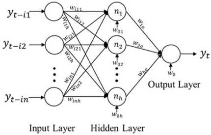
Fig.1. Structure of the ANN to forecast a univariate time series

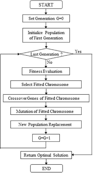
Fig.2. Flow chart of Genetic Algorithm

• C.    Genetic Algorithm

Genetic Algorithm (GA) is an algorithm to find the optimal solution and it was introduced by John Holland [18]. The concept of GA comes from the evolution theory and the steps of GA starts with generating an initial set of random solutions called population. Each solution in the population is represented in encoded form and is called a chromosome. Each chromosome consist of a sequence of genes which represent the parameters to be optimized. After that, each chromosome will be evaluated by a fitness evaluation function and the fitted chromosome will be selected to be a member of the next generation in the selection operation. The fitted chromosome will be operated with two genetic operators, namely crossover and mutation, to avoid the local optimum solution. The last step of GA in each iteration is to replace the old population with a new better fitted population. The process of GA to find the optimum solution will be done iteratively until the last population is met and the best solution is returned to represent the optimum solution. A flowchart of GA can be shown as figure 2.

• IV.    Methodology

This research aims to study and develop a univariate time series forecasting model by using the Artificial Neural Network (ANN) with a Feed Forward Back Propagation algorithm to generate a forecasting model and we determine the structure of ANN with the Autoregressive (AR) form and Genetic Algorithm (GA). The AR form is used to choose the lag time observed values to be an input of the ANN model. The GA is used to determine the number of neurons in the hidden layer of the ANN model. Three ANN models with 1 to 3 hidden layers are determined to experiment. We evaluate our experiment by comparing the forecasting accuracy between three ANN models and the ARIMA model with error measurement by Root Mean Square Error (RMSE) and Mean Absolute Percentage Error (MAPE). The equation of RMSE and MAPE can be shown as equation 4 and 5 [19] respectively.

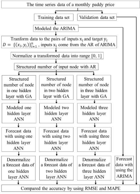
Fig.3. Experimental procedure

n ^

Rmse = a - E (y. — y* )2              (4)

«“

MAPE = ^- )E 100 y * y * n 7=1         У *

Where, y equal to an actual observed value at time t y ˆ equal to a forecasting value at time t n equal to a number of time periods to forecast

Two experimented datasets are in the form of a univariate time series and the monthly paddy price in Thailand. These datasets were published in the official website of the Office of Agricultural Economics in the Ministry of Agriculture and Cooperatives, Thailand. The first dataset is a monthly price of Jasmine paddy and the second dataset is a monthly price of paddy with moisture 15%. Each dataset is a monthly data, since Jan 1997 to Dec 2017 with a number of observed values equal to 252 values. Therefore, our work is a long term forecasting similar to some prior researches such as a research of Wang et. Al. [20] that used the 31 data points of the annual total electricity consumption of Beijing city during between 1978 and 2008 to generate the forecasting model. This includes a research of Kaytez et. Al. [21] that used the 40 data points of the annual electricity consumption of Turkey during between 1970 and 2009 to generate the forecasting model.

We experimented each dataset with the same procedure and used R language as an experimental tool. Our experimental procedure can be shown as figure 3 and the step of our experimental procedure can be described as follows.

• 1.    Generate a univariate time series with a monthly time period from observed values which is a monthly paddy price.

• 2.    Divide a time series into a training set to train each forecasting model and a validation set to evaluate an accuracy of the model. A training set is the data, since Jan 1997 to Dec 2016 with a number of observed values equal to 240 values and a validation set is the data in the last year (2017) with a number of observed values equal to 12 values.

• 3.    A time series training set has a monthly time period with 12 months per year or 12 time periods per season. In R language, there is a function which named “auto.arima()” in the “forecast” package that is authored by Rob Hyndman and is published in the library repository of R. This function is used to determine a suitable ARIMA(p, d, q)x(P, D, Q) S (when S=12). It returns the suitable value of parameters, namely p, d, q and P, D, Q by measuring the Akaike information criterion (AIC).

• 4.    Generate the suitable ARIMA model by using the “arima()” function in the “forecast” package.

• 5.    Transform a time series training set to be a pair of

• 6.  Normalize data to be an interval value of 0 to 1.

• 7.  Determine inputs of the ANN, which is lag time

• 8.    Searching a suitable number of neurons in the hidden layer, when the hidden layer is 1 to 3 layers by using the Genetic Algorithm. In R, there is a function to find the optimum solution followed by an algorithm of GA, and this function is the “rgba()” function available in the “genalg” package that is authored by Egon Willighagen and Michel Ballings. The chromosome of GA is the number of neurons in the hidden layer and set a scope to search number of neurons from 1 to 20 neurons with 50 generations and 100 chromosomes in each generation. The pseudo code to find the optimum number of neurons followed by an algorithm of GA can be shown as figure 4.

• 9.    Generate three ANN model with 1 to 3 hidden layers, when the optimum number of neurons in hidden layer come from GA. To generate the ANN model, we used the “neuralnet()” function in the “neuralnet” package that was authored by Stefan Fritsch et al.

• 10.    Forecast data from three ANN model.

• 11.    Denormalize a forecasting data to be its normal value.

• 12.    Forecast data from the ARIMA model.

• 13.    Compare the forecasting accuracy of three ANN and ARIMA model by measuring RMSE and MAPE.

input vector ( x ) and output ( y ), when x is determined by the Autoregressive form of ARIMA.

observed values that come from the analysis of the Autoregressive form.

Function of fitness evaluation(chromosome) (

Return value = NA

Generate neural network model with a chromosome

Forecast data with neural network model

Calculate MAPE when MAPE is a fitness evaluation

Return value = MAPE }

GA result=rbga(MinNeuron=l, MaxNeuron=2 0, popSize= 100, iters=50, evalFunc=Fimction of fitness evaluation) Summarize GA result

Fig.4. Pseudo code to find the optimum number of neurons

• V.    Results and Discussion

Our research presents a forecasting model by using the Artificial Neural Network technique and determine its structure with Autoregressive form and Genetic Algorithm, it’s called that AR-GA-ANN model. We generate three AR-GA-ANN models with 1 to 3 hidden layer and ARIMA model to experiment with two datasets in the same procedure and the result can be shown as follows.

• A.    The result of the Autoregressive analysis to define inputs of AR-GA-ANN model

To define inputs of AR-GA-ANN model by using the

Autoregressive analysis, we start with a searching for a suitable ARIMA formation by using the “auto.arima()” function. This function evaluates a suitable ARIMA formation by measuring the AIC that is approximate variance of Kullback Leibler Information between an actual formation and a suitable formation. A suitable formation is a formation that has minimum AIC. The result of an experiment indicates that a suitable ARIMA formation of two datasets can be shown as figure 5.

When we know a suitable ARIMA formation of each dataset, we adopt it to analyze the Autoregressive form of each dataset with an equation 1. The result analysis can be shown as follows

• 1.    The first dataset is a dataset of a Jasmine paddy and its suitable ARIMA formation is an ARIMA(2, 1, 0)(1, 0, 0) 12 . Therefore, we represent p=2, d=1, P=1 and S=12 into equation 3 as follows.

• 2.    The second dataset is a dataset of a paddy with

(1-θB-θB2)(1- ΘB12)(1-B)y =MA (1-B-θB+θB2-θB2+θB3-ΘB12+ΘB13+ θΘB13-θΘB14+θ ΘB14-θ ΘB15)y =MA yt = (1+θ1) yt-1 -(θ1 -θ2)yt-2 -θ2yt-3 +Θ1yt-12-

( Θ 1 + θ 1 Θ 1 ) y t - 13 + ( θ 1 Θ 1 - θ 2 Θ 1 ) y t - 14 + θ 2 Θ 1 y t - 14 + MA

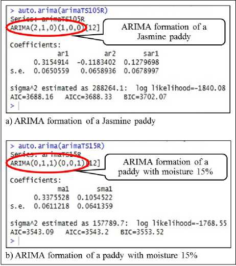
Fig.5. ARIMA formation of each dataset

From equation 6, we conclude that the inputs of AR-GA-ANN model consists of lag time values at time t-1,    t-2,    t-3,    t-12,    t-13,    t-14 and t-15

( yt-1 , yt-2, yt-3, yt-12, yt-13, yt-14, yt-15). Therefore, the first dataset has a number of input nodes equal to 7 nodes.

moisture 15% and its suitable ARIMA formation is an ARIMA(0, 1, 1)(0, 0, 1) 12 . Therefore, we represent d=1 and S=12 into equation 3, while we ignore q=1 and Q=1 because they are a component of Moving Average (MA), as follows.

(1 - B) y t = MA yt = y,-1 + MA                 (7)

From equation 7, we conclude that the inputs of AR-GA-ANN model consists of only one lag time value at time t-1 ( y ). Therefore, the second dataset has a number of input nodes equal to 1 node.

• B.    The result of Genetic Algorithm to determine the number of neurons in the hidden layer

To determine the number of neurons in the hidden layer, we use the GA to find the optimal number of neurons of three AR-GA-ANN model. This result can be shown as figure 6-7 and can be concluded as shown in table 1.

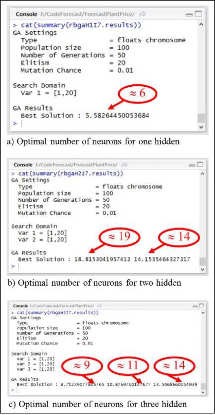
Fig.6. Optimal number of neurons for the first dataset

Table 1. Optimal number of neurons in the hidden layer

Dataset	One Hidden	Two Hidden	Three Hidden
The 1st dataset (Jasmine paddy)	6	19, 14	9, 11, 14
The 2nd dataset (paddy with moisture 15%)	2	2, 11	8, 15, 18

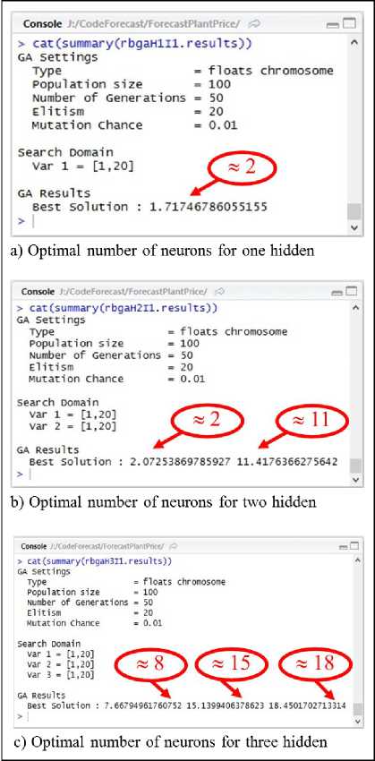
Fig.7. Optimal number of neurons for the second dataset

• C.    The result of model accuracy and performance

  As we know the optimal structure of three AR-GA-ANN models, which have the number of hidden layers in 1 to 3 layers, we generate three AR-GA-ANN models by using a training set. After that, we use each AR-GA-ANN model to forecast 12 observed values that are monthly prices of paddy in 2017 and use 12 forecasting values to compare with 12 actual values in the same time periods by error measuring with RMSE and MAPE. Finally, we compare the RMSE and MAPE of three AR-GA-ANN models together with the ARIMA model. Our experimental result found that all of AR-GA-ANN models have lower RMSE and MAPE than

  ARIMA model and the AR-GA-ANN model that has the lowest error is the AR-GA-ANN with one hidden layer and each dataset has the same result. Therefore, the optimal forecasting model to forecast a monthly price of paddy in Thailand is the AR-GA-ANN with one hidden layer and the structure of the optimal AR-GA-ANN can be shown as figure 8-9. In figure 8, the ANN model for the first dataset was trained at 544 epochs and it has a sum square error (SSE) equal to 0.18073. In figure 9, the ANN model for the second dataset was trained at 384 epochs and it has a sum square error (SSE) equal to 0.251745. The error in figure 8-9 is a sum of error in the training process, but it is not an error of a validation dataset that is measured by the RMSE and MAPE. The RMSE and MAPE of each model can be shown in table 2. When we plot a graph of forecasting values comparing with actual values to detect a movement of data, our result found that a forecasting graph of AR-GA-ANN is similar and align with a graph of actual values, but a forecasting graph of ARIMA is not similar or not align with a graph of actual value and both of dataset have the same result. Therefore, The AR-GA-ANN can detect a movement of data better than ARIMA and a graph of each dataset can be shown as figure 10-11.

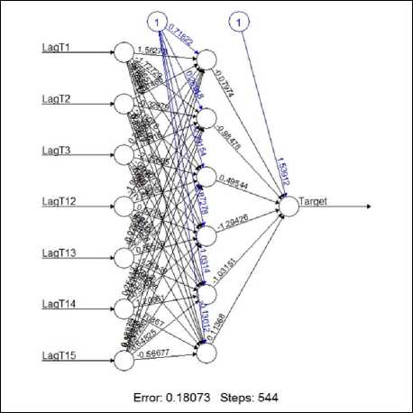
Fig.8. Optimal structure of AR-GA-ANN for the first dataset

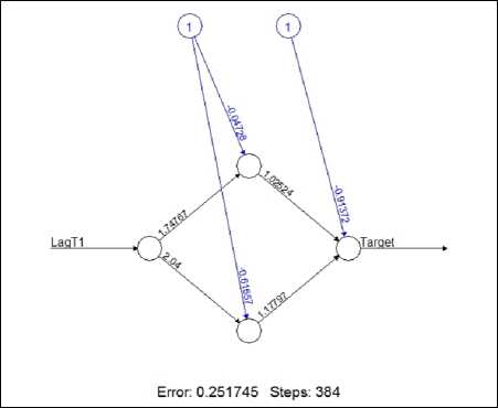
Fig.9. Optimal structure of AR-GA-ANN for the second dataset

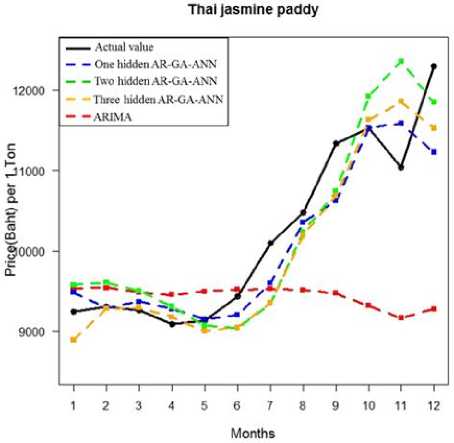
Fig.10. Comparison graph of the first dataset

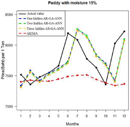
Fig.11. Comparison graph of the second dataset

Table 2. Result of RMSE and MAPE

Dataset	One hidden AR-GA-ANN		Two hidden AR-GA-ANN		Three hidden AR-GA-ANN		ARIMA
	RMSE	MAPE	RMSE	MAPE	RMSE	MAPE	RMSE	MAPE
The 1st dataset	446.40	2.90	543.73	4.23	469.11	3.45	1378.06	9.08
The 2nd dataset	291.83	3.01	304.34	3.20	294.45	3.07	432.94	4.10

• VI. Conclusions

This research studies a development of the forecasting model based on the Artificial Neural Networks (ANN) technique by presenting a novel method to determine the optimal structure of ANN. The optimal structure of ANN is determined by using the Autoregressive component of the ARIMA model to define input nodes of the ANN and using the Genetic Algorithms (GA) to define a number of neurons in the hidden layer. We use two datasets in the form of a univariate time series and a monthly paddy price in Thailand. We experiment with both of the dataset in the same procedure and evaluate our experiment by error measuring with RMSE and MAPE. Our result found that the optimal ANN of the first dataset has a network structure of 7-6-1 and the optimal ANN of the second dataset has a network structure of 1-2-1. When we evaluate our experiment by error measurement, the results found that all of ANN models have lower RMSE and MAPE than the ARIMA model and the ANN with one hidden layer has lowest RMSE and MAPE in both datasets. This result is consistent with a prior research of Wang and Meng [22] which experiment by generating the ANN with one hidden layer to avoid the overfitting problem and their result found that the ANN with one hidden layer has the lowest error same as our result. Therefore, we can conclude that our approach to determine the optimal structure of ANN can generate a model to forecast a monthly paddy prices in Thailand precisely.

In future, our approach to determine the optimal structure of ANN may be applied to some other well-known ANNs/ DNNs to test whether our approach is applicable to other ANNs/ DNNs.

Acknowledgment

We are grateful to Nakhon Ratchasima Rajabhat University for funding this research and wish to thank the Office of Agricultural Economics (Thailand) for publicizing the data that had been used in this study.