Determination of status of family stage prosperous of Sidareja District using data mining techniques

Published Online October 2018 in MECS

• I.    Introduction

  The prosperous Family according to law no. 10 of 1992 are families formed on legitimate marriages, able to meet the needs of a proper spiritual and material life, devoted to God the ALMIGHTY, has a matching relationship, aligned, and balanced between Member and

  among families with society and the environment [1]. Implementation of Family Data Collection in 2015 Sidareja District has conducted family data collection using F / I / MDK / 08 form. The family data updating toolkit (MDK) or F / I / MDK / 08, contains complete family data variables in one sheet for each family. With this MDK form the family data is collected by the collecting cadres with PLKB / PKB, then collected at the Regency / City level for subsequent recording and processing. Data collection of sub-field of KS assisted PLKB (Family Planning Officer) sub-district to do socialization directly through KB office, PP, PA. Any data gained in the activity will show the level of family welfare.

The amount of data relating to the level of family welfare collected contains various types of knowledge useful for processing decision-making, such as those related to the classification or grouping data to the levels specified above, but the pattern of data and knowledge is very difficult to be discovered by analyzing manually. In this case data mining can be used to determine the status of the prosperous family stage. Data mining is basically a component of the Knowledge Discovery Process. As one expert puts it, Merely finding patterns is not enough. You must respond to the patterns and act on them, ultimately turning data into information, information into action, and action into value. This is the virtuous cycle of data mining in a nutshell. The main goal of this analysis process is to take information from a data set and convert it into an understandable and meaningful structure for further use. Data Mining is used for solving problems by analyzing data that is present in the databases [2]. In this study the authors will compare two methods in data mining techniques namely Naive Bayes method, KNN method and with the addition of PCA feature selection to obtain the most accurate test in data processing in determining the status of family stages prosperous District Sidareja.

The remainder of this paper is organized as follows: Section 2 describes related work. Section 3 explains the research method used. Section 4 describes how the Naive Bayes method, the KNN method, and the PCA method can solve the problems in this paper and section 5 describes conclusions and future work are given in the final section.

• II.    Related Work

The researches in [3] in this study, Fuzzy Naïve Bayes classifier is proposed for automatic text categorization. Here the most important features are selected for each classes those features are termed as class-specific features. The class specific features reduced the dimensionality of features and it speed up the process of Fuzzy Naïve Bayes classifier. The texts are categorized by combining the fuzzy rule with Bayesian classification which facilitates improvement in the probabilities of each of the classes by considering many of the features that are left un-classified or incorrectly classified by applying the Bayesian classification alone. The experimental results proved that the proposed Fuzzy Naïve Bayes classifier has high accuracy.

Researches being done by [4] is using KNN algorithm in the process of face recognition on ARM processor. Proposed algorithm tested on three datasets which is Olivetti Research Laboratory (ORL), Yale face and the proposed algorithm being implemented on ARM11 700MHz. 10-fold cross-validation showing that KNN face recognition detect 91.5% face with k=1. Overall the research showing that algorithm proposed able to recognize face on 2.66 seconds ARM processor.

The researchers in [5] explain proposed model consists of two stages, the first stage is to determine the news polarities to be either positive or negative using naïve Bayes algorithm, and the second stage incorporates the output of the first stage as input along with the processed historical numeric data attributes to predict the future stock trend using KNN algorithm. The results of our proposed model achieved higher accuracy for sentiment analysis in determining the news polarities by using Naïve Bayes algorithm up to 86.21%. In the second stage of analysis, results proved the importance of considering different values of numeric attributes. This achieved the highest accuracy compared to other previous researches, our model for predicting the future behavior of stock market obtained accuracy up to 89.80%. [6] Sentiment analysis considered a particularbranch of data mining that classifies textual data into positive, negative and neutral sentiments.

The researches in [7] this paper for Sentiment Analysis we are using two Supervised Machine Learning algorithms: Naive Bayes and KNN to calculate the accuracies, precisions (of positive and negative corpuses) and recall values (of positive and negative corpuses). The difficulties in Sentiment Analysis are an opinion word which is treated as positive side may be considered as negative in another situation. Also the degree of positivity or negativity also has a great impact on the opinions. For example “good” and “very good” cannot be treated same.

The researchers in [8] explain evaluate the performance for sentiment classification in terms of accuracy, precision and recall. This research, we compared two supervised machine learning algorithms of Naïve Bayes‘ and KNN for sentiment classification of the movie reviews and hotel reviews. The experimental results show that the classifiers yielded better results for the movie reviews with the Naïve Bayes‘ approach giving above 80% accuracies and outperforming than the KNN approach. However for the hotel reviews, the accuracies are much lower and both the classifiers yielded similar results.

Researches being done by [9] In the process classification models the KNN algorithm were able to see improvements in their accuracy rates. Although the KNN model had no improvement with regards to accuracy, the true benefit was in the reduction of storage space needed for the modeling and classifying of data. This lead to a reduction in the time needed to for processing, which is pivotal for a very time consuming algorithm.

The researchers in [10] explain that KNN was applied to classify the monogenean specimens based on the extracted features. 50% of the dataset was used for training and the other 50% was used as testing for system evaluation. Our   approach demonstrated overall classification accuracy of 90%. In this study Leave One Out (LOO) cross validation is used for validation of our system and the accuracy is 91.25%.

The researchers in [11] explain that a Naive Bayes classification with Rsa cryptosystem as an alternative to KNN classification with Paillier cryptosystem. Experiments on a large number of datasets show that the proposed system has given the result with more accuracy, effective and encryption time consumes very less compared to existing system. We plan to investigate alternative and more efficient solutions to the Security problem in our future work. Also, we will investigate and extend our research to other classification algorithms.

• III.    Research Methods

The research method used is descriptive analysis method with quantitative approach means that the research done is emphasizing the analysis on numerical data (number), which aims to get a clear picture of a state based on data obtained by presenting, collecting and analyzing the data so it becomes new information that can be used to analyze the problem under investigation. The research method applied in this research can be seen in Fig. 1 below:

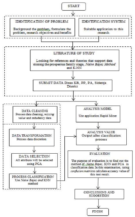
Fig.1. Research Workflow

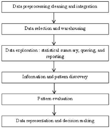
Fig.2. Knowledge discovery steps

There are a lot of requirements and challenges in data mining that should be taken in consideration before using data mining algorithms, the first thing to study that the algorithm can handle different types of data , the second is that the algorithm can extract useful information from a huge amount of data efficiently, the third is to check how much the information discovered by the algorithm is valuable and useful and the next is to see if the algorithm can do mining over different sources of data , the last thing is the protection of user data and if the algorithm provides privacy [14].

The Naive Bayes algorithm is a simple probabilistic classifier that calculates a set of probabilities by counting the frequency and combinations of values in a given data set. The algorithm uses Bayes theorem and assumes all attributes to be independent given the value of the class variable. This conditional independence assumption rarely holds true in real world applications, hence the characterization as Naive yet the algorithm tends to perform well and learn rapidly in various supervised classification problems [15]. Naïve Bayes Classifier is a term dealing with simple probabilistic classifier based on applying Bayes Theorem with strong independence assumptions. It assumes that the presence or absence of particular feature of a class is unrelated to the presence or absence of any other feature [16].

The Naive Bayes algorithm is based on conditional probabilities. It uses Bayes' theorem, a formula that calculates a probability by counting the frequency of values and combinations of values in the historical data. Bayes' Theorem finds the probability of an event occurring given the probability of another event that has already occurred. If B represents the dependent event and A represents the prior event, Bayes' theorem can be stated as follows. Prob (B given A) = Prob (A and B) / Prob (A). To calculate the probability of B given A, the algorithm counts the number of cases where A and B occur together and divides it by the number of cases where A occurs alone [17].

KNN being done by find the nearest (most similar) group of k object in the data training with the object in the new dataset or testing data [18]. To validate a sample point in the train set, the H nearest neighbors of the point is considered. Among the H nearest neighbors of a train sample x, validity(x) counts the number of points with the same label to the label of x. Equation 1 is the formula which is proposed to compute the validity of every points in train set

Validaty(x) = -If₌₁S(lblG)»lbl(NU))) (1)

Where H is the number of considered neighbors and lbl(x) returns the true class label of the sample x. also, Ni(x) stands for the ith nearest neighbor of the point x. The function S takes into account the similarity between the point x and the ith nearest neighbor. Equation 2 defines this function [19].

^» = fi ^a_QV_b (2)

The KNN algorithm is a technique for classifying objects based on the next training data in the feature space. It is among simplest of all mechanism learning algorithms. The algorithm operates on a set of d-dimensional vectors,

D = {xi | i = 1...Я)            (3)

where x _i ∈ k ^d denotes the i the data point. The algorithm is initialized by selection k points in k ^d as the initial k cluster representatives or “centroids”. Techniques for select these primary seeds include sampling at random from the dataset, setting them as the solution of clustering a small subset of the data or perturbing the global mean of the data k times. Then the algorithm iterates between two steps till junction [20]:

• 1.    Data Assignment each data point is assign to its add join centroid, with ties broken arbitrarily. This results in a partitioning of the data.

• 2.    Relocation of “means”. Each group representative is relocating to the center (mean) of all data points assign to it. If the data points come with a possibility measure (weights), then the relocation is to the expectations (weighted mean) of the data partitions.

PCA is a method of data processing consisting in the extraction of a small number of synthetic variables, called principal components, from a large number of variables measured in order to explain a certain phenomenon. Principal components are a sequence of projections of the data, mutually uncorrelated and ordered in variance which are obtained as linear manifolds approximating a set of N points [21]. PCA is a well-known technique for data exploration and dimensionality reduction. The goal of PCA is to represent a centered data matrix as a linear combination of few basis vectors. In the classical deterministic setting, factors are extracted as orthonormal vectors that maximize the explained variance in the data matrix. Beyond classic PCA, various extensions have been proposed that incorporate sparsity and other domain structure, or are designed to incorporate useful statistical properties such as noise tolerance in high dimensions [22].

This method uses the matrix table as in Table 1 if the data set consists of only two classes, one class is considered positive and the other negative.

Table 1. Model Confusion Matrix [23]

Correct classifications	Classified as
	+	-
+	True Positives	False Negatives
-	False Positives	True Negatives

True positives are the number of positive records classified as positive, false positives is the number of negative records classified as positive, false negatives is the number of positive records classified as negative, true negatives is the number of negative records classified as negative, then enter the test data. After the test data is inserted into the confusion matrix, compute the values that have been entered to calculate the number of sensitivity (recall), specificity, precision and accuracy [23].

Sensitivity is used to compare the number of TP against the number of positive records while the specificity is the ratio of the number of TN to the number of negative records. To calculate used equation below [24]:

Recall, True Positive Rate (Sensitivity):

TP _ TP P ~ TP+FN

Recall, True Negative Rate (Specificity):

TN _ TN N TN+FP

Precision, Positive Predictive Value (PPV):

TP

TP+FP

Precision, Negative Predictive Value (NPV):

TN

TN+FN

Accuracy:

TP+TN

TP+ FP + TN+FN

Information :

TP = the number of true is positive

TN = true negative count

P = number of positive records

N = the number of tuples is negative

FP = number of false positive

FN = number of false negatives

• IV.    Result and Discussion

The first step is to Data Collection and Information,

Data collected by UPT KB, PP, PA Sidareja District on the determination of the status of prosperous family stages referring to the Decree of State Minister of Women Empowerment / Head of BKKBN number 21 of 1994 on the implementation of Prosperous Family Development. The data obtained from the family data (DK) form that has been filled by field officers who directly go to each family. The first step begins with the determination of the attributes of the DK form to be used, in table 2 as follows:

Table 2. Attribute Family Welfare

Attribute	Description
Family	Is a Family Name
Indicator 1 (A)	Generally family members eat twice a day or more
Indicator 2 (B)	Family members have different clothes for at home, work / school and traveling
Indicator 3 (C)	House occupied by the family has a good roof, floor, wall
Indicator 4 (D)	If any member of the sick family is taken to a health facility
Indicator 5 (E)	If the fertile age couple wishes to go to the contraceptive service means go to contraceptive services
Indicator 6 (F)	All children aged 7-15 years in the family attend school
Indicator 7 (G)	Generally family members perform worship according to their respective religions and beliefs
Indicator 8 (H)	At least once a week all family members eat meat / fish / eggs
Indicator 9 (I)	All family members earn at least one pair of new clothes a year
Indicator 10 (J)	House floor area of at least 8 m2 for each occupant of the house
Indicator 11 (K)	The last three months of the family are in good health, so they can perform their respective duties / functions
Indicator 12 (L)	There is one or more family members working to earn an income
Indicator 13 (M)	All family members aged 10 - 60 years can read Latin script
Indicator 14 (N)	A couple of childbearing age with two or more children using contraceptive devices / drugs
Indicator 15 (O)	The family seeks to increase religious knowledge
Indicator 16 (P)	Part of family income is saved in money or in kind
Indicator 17 (Q)	Family eating habits together at least once a week are used to communicate
Indicator 18 (R)	The family participates in community activities in the neighborhood
Indicator 19 (S)	The family obtains information from newspapers / magazines / radio / TV
Indicator 20 (T)	The family regularly voluntarily contributes material for social activities
Indicator 21 (U)	There are active family members as administrators of social associations / foundations / community institutions
Status (class)	Is a family status consisting of: Pre Prosperous; Family welfare I (KS I); Family welfare II (KS II); Family welfare III (KS III); Family welfare III+ (KS III +)

From table 2 the attributes used as the determinant variable are Indicator 1 to 21, while the objective variable is the status (class) with Pre-prosperous attribute value, KS I, KS II, KS III and KS III +.

Second process is data cleaning in this research is done manually, because the raw data in the form of paper printing, so the process of cleaning the data is done outside the application. Data is cleared of some items that have no value, only data that has complete attributes and meets the requirements of the selected needs. Data used as many as 920 data of prosperous families consists of 18 different RTs in 10 villages. After cleaning the data and having complete attribute only 810 data of prosperous family.

The third process is data transformation is used to change the dataset so that the best information content is retrieved and by reducing or changing the standard data type so that data is ready for use to be presented to data mining techniques using Rapid Miner.

The fourth process is the process of selecting a data set variable using the PCA method by matching the initial variables / attributes with the variables / attributes present in the base case. The result of feature selection based on PCA can be seen in Table 3. In each feature selection method it produces different feature

Table 3. Results of feature selection based on PCA

Feature Selection Method	Attributes / features
PCA	Feature 1, Feature 2, Feature 3, Feature 4, Feature 5, Feature 6, Feature 7, Feature 8, Feature 9, Feature 10, Feature 11, Feature 12, Feature 13

Based on Table 3, number of features selected by the PCA method as many as 13 attributes or features are selected, the PCA method will transform the feature on the dataset of new feature form, so in this study it is named Feature 1, Feature 2, Feature 3, Feature 4, Feature 5, Features 6, Feature 7, Feature 8, Feature 9, Feature 10, Feature 11, Feature 12, Feature 13. Selected attributes or features will be used in the next process that is the classification process, while the unselected features will be deleted along with the data from the dataset, so that there are 8 attributes along with the deleted data from the dataset used.

The Fifth process is classification is important for management of decision making. Given an object, assigning it to one of predefined target categories or classes is called classification. The goal of classification is to accurately predict the target class for each case in the data [25].

At the classification stage, the specified dataset is then imported for subsequent training and testing process with the proposed algorithm, first using Naïve Bayes and the second KNN algorithm. In the training column there is a classification algorithm that is implemented, the Naïve Bayes algorithm as and KNN algorithm. While in the 'Testing' column there is 'Apply Model' to run the selected algorithm model and 'Performance' to measure the performance / performance of each algorithm mode.

The sixth process is evaluation, Furthermore in this phase Algorithm Naive Bayes, KNN and PCA for the classification of prosperous family stages can be done in several steps. First, in this study the system performance is based on confusion matrix for each type / level for models using Naive Bayes, KNN, PCA + Naive Bayes, and PCA + KNN, as shown in Table 4 to Table 7. Second, from confusion matrix results of each type / level, then measure performance based on sensitivity, specificity, precision and accuracy. Additionally the average for each class is shown as shown in Table 8 Average performance is the average value of all types / levels for the same model and performance.

Table 4. Confusion Matrix for Naive Bayes Algorithm

A	B	C	D	E	Classified as
196	30	0	0	0	Pred A = KS I
1	135	3	0	0	Pred B = KS II
0	0	145	0	0	Pred C = KS III
0	0	0	0	0	Pred D = KS III +
3	0	0	1	296	Pred E = Pre Prosperous

In Table 4 The results of the classification of the welfare family dataset using the Naive Bayes algorithm obtained the test results from 810 data, 196 were classified KS I according to prediction, 30 data were predicted KS I but the result was KS II. 1 data predicted KS II was the result of KS I, 135 data classified KS II in accordance with predictions. 3 KS II prediction data but it turns out KS III. 145 data KS III In accordance with the prediction, 3 data prediction pre prosperous results KS I, 1 data prediction pre prosperous results KS III +, 296 data classified pre prosperous in accordance with predictions.

Table 5. Confusion Matrix for KNN Algorithm

A	B	C	D	E	Classified as
189	7	0	0	0	Pred A = KS I
11	158	3	0	0	Pred B = KS II
0	0	145	1	1	Pred C = KS III
0	0	0	0	0	Pred D = KS III +
0	0	0	0	295	Pred E = Pre Prosperous

Table 5 is the result of the classification of the prosperous family dataset by using the KNN algorithm obtained test results from 810 data, 189 KS I classified according to prediction, 7 data predicted KS I but the result is KS II. 11 data predicted KS II was the result of KS I, 158 data classified KS II in accordance with its prediction, 3 data prediction KS II but it turned KS III. 145 KS III data In accordance with the prediction, 1 KS III prediction data was KS III + result, 1 KS III prediction data was the result of pre prosperous, 295 data classified pre prosperous according to prediction.

Table 6. Confusion Matrix for Naive Bayes + PCA Algorithm

A	B	C	D	E	Classified as
190	7	0	0	0	Pred A = KS I
1	148	3	0	0	Pred B = KS II
0	1	130	0	0	Pred C = KS III
0	0	0	0	0	Pred D = KS III +
9	9	15	1	296	Pred E = Pre Prosperous

Table 6 is the result of classification on the dataset of prosperous families using Naive Bayes + PCA algorithm obtained test results from 810 data, 190 KS I classified according to prediction, 7 data predicted KS I but the result is KS II. 1 data predicted KS II was the result of KS I, 148 data classified KS II in accordance with predictions. 3 KS II prediction data but it turns out KS III. 1 KS III predicted data resulted KS II, 130 KS III data in accordance with predictions, 9 data prediction pre prosperous results KS I, 9 data pre-prosperous prediction was the result of KS II. 15 pre-prosperous prediction data was the result of KS III. 1 data pre-prosperous prediction was the result KS III +. 296 data are classified pre prosperous according to prediction.

Table 7. Confusion Matrix for KNN + PCA Algorithm

A	B	C	D	E	Classified as
190	7	0	0	0	Pred A = KS I
10	158	0	0	0	Pred B = KS II
0	0	145	1	0	Pred C = KS III
0	0	0	0	0	Pred D = KS III +
0	0	0	0	296	Pred E = Pre Prosperous

Table 7 is the result of classification in prosperous family dataset by using KNN + PCA algorithm obtained test result from 810 data, 190 classified KS I according to prediction, 7 data predicted KS I but it turns out KS II result. 10 data predicted KS II was the result of KS I, 158

data classified KS II in accordance with predictions. 145 KS III data in accordance with the prediction. 1 prediction data KS III turns out the result KS III +, 296 data classified pre prosperous in accordance with the

Table 8. Confusion Matrix classification in each class

No	Method	Classification	Class
			A	B	C	D	E
1	Naive Bayes	True Positive (TP)	196	135	145	0	296
		True Negative (TN)	580	641	662	809	510
		False Positive (FP)	4	30	3	1	0
		False Negative (FN)	30	4	0	0	4
2	KNN	True Positive (TP)	190	158	145	0	295
		True Negative (TN)	603	632	660	809	514
		False Positive (FP)	10	7	3	1	1
		False Negative (FN)	7	13	2	0	0
3	Naive Bayes + PCA	True Positive (TP)	190	148	130	0	296
		True Negative (TN)	603	641	661	809	480
		False Positive (FP)	10	17	18	1	0
		False Negative (FN)	7	4	1	0	34
4	KNN + PCA	True Positive (TP)	190	158	145	0	296
		True Negative (TN)	603	632	661	809	514
		False Positive (FP)	10	7	3	1	0
		False Negative (FN)	7	13	1	0	0

TN

Table 8 is the result of the classification of the welfare family dataset using the Naïve Bayes, KNN, Naïve Bayes + PCA, KNN + PCA algorithm. Based on the confusion matrix obtained, the values of TP, TN, FP, and FN will be obtained for each class. From the test data that has been obtained, then calculate the value of performance sensitivity (recall), specificity, precision positive predictive value, negative predictive value and accuracy. Calculation on KS I class by using Naive Bayes Algorithm method, KNN, Naive Bayes + PCA, KNN + PCA for performance value =

TP 196

• 1.    Sensitivity (recall) =                        =

86.73 % prediction. Based on the confusion matrix obtained, the values of TP, TN, FP, and FN will be obtained for each class as follows:

.y

Specificity =                = 99.32 %

• ^{r 3} TN+FP 580+4

• 3.    PPV =-----= ---- = 98 %

• 4.    NPV = TN+FN 580+ 30 = 95.08%

• 5.    Accuracy =

TP 196

.

TN      530

TP+TN

3 TP+FP+TN+FN

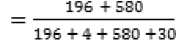
= 95.80 %

Calculation values of sensitivity, specificity, PPV, NPV and accuracy are found in Table 9.

Table 9. Sensitivity, Specificity, PPV, NPV and Accuracy scores

Class	Method	Sensitivity	Specificity	PPV	NPV	Accuracy
A = KS I	Naive Bayes Algorithm	86.73 %	99.32 %	98.00 %	95.08 %	95.80 %
	KNN Algorithm	96.42 %	98.20 %	94.5 %	98.85 %	97.77 %
	Naive Bayes + PCA Algorithm	96.45 %	98.37 %	95.00 %	98.85 %	97.90 %
	KNN + PCA Algorithm	96.45 %	98.37 %	95.00 %	98.85 %	97.90 %
B = KS II	Naive Bayes Algorithm	97.12 %	95.53 %	81.82 %	99.38 %	95.80 %
	KNN Algorithm	91.86 %	98.90 %	95.76 %	97.83 %	97.4 %
	Naive Bayes + PCA Algorithm	97.37 %	97.42 %	89.70 %	99.38 %	97.41 %
	KNN + PCA Algorithm	92.40 %	98.90 %	95.76 %	97.98 %	97.53 %
C = KS III	Naive Bayes Algorithm	100.00 %	99.55 %	97.97 %	100.00 %	99.63 %
	KNN Algorithm	98.64 %	99.55 %	97.97 %	99.69 %	99.38 %
	Naive Bayes + PCA Algorithm	99.24 %	97.35 %	87.84 %	99.85 %	97.65 %
	KNN + PCA Algorithm	99.32 %	99.55 %	97.97 %	99.85 %	99.51 %
D = KS IIII +	Naive Bayes Algorithm	0.00 %	99.88 %	0.00 %	100.00 %	99.88 %
	KNN Algorithm	0.00 %	99.88 %	0.00 %	100.00 %	99.88 %
	Naive Bayes + PCA Algorithm	0.00 %	99.88 %	0.00 %	100.00 %	99.88 %
	KNN + PCA Algorithm	0.00 %	99.88 %	0.00 %	100.00 %	99.88 %
E = Pre Prosperous	Naive Bayes Algorithm	98.67 %	100.00 %	100.00 %	99.22 %	99.51 %
	KNN Algorithm	100.00 %	99.80 %	99.66 %	100.00 %	99.88 %
	Naive Bayes + PCA Algorithm	89.70 %	100.00 %	100.00 %	93.39 %	95.80 %
	KNN + PCA Algorithm	100.00 %	100.00 %	100.00 %	100.00 %	100.00 %
Average	Naive Bayes Algorithm	76.50 %	98.85 %	75.56 %	98.74 %	98.12 %
	KNN Algorithm	77.38 %	99.27 %	77.58 %	99.27 %	98.86 %
	Naive Bayes + PCA Algorithm	76.55 %	98.60 %	74.51 %	98.29 %	97.73 %
	KNN + PCA Algorithm	77.63 %	99.34 %	77.75 %	99.34 %	99.35 %

• V. Conclusion

The aim of study is to evaluate the performance sentiment classification in terms of accuracy. In this paper, we compared two machine learning algorithms of Naïve Bayes‘ and KNN to determining the prosperous family stage of Sidareja District.

The result of the performance of classification algorithm for the case of determining the status of prosperous family stages for Naïve Bayes algorithm using confusion matrix obtained 98.12% accuracy after the selection added PCA feature to 97.73% while the KNN algorithm obtained accuracy of 98.86%, then after added selection PCA features increased to 98.96%.

With the addition of PCA feature selection the Naïve Bayes algorithm of accuracy decreased from 98.12% to 97.73% while the KNN algorithm added PCA feature selection of accuracy increased from 98.86% to 98.96%. So with the addition of PCA feature selection does not affect the calculation accuracy too much.

Than the performance of the KNN algorithm is superior to the Naïve Bayes algorithm in the case of determining the status of the prosperous family stage. This is evident from the use of confusion matrix in measuring performance value based on sensitivity (recall), specificity, precision Positive Predictive Value, Negative Predictive Value and accuracy obtained by each algorithm.

For further work we would like to to use other classification algorithms and use selection of features other than PCA to obtain accurate and optimal results and the use of different variables for the same case. The use of PCA method feature selection in this study has an effect on the attributes used, this is because the PCA method transforms the dataset attribute into less. The Feature Selection by the PCA method can be used if the attributes used are not bound by the applicable rules. The results of this study using Naïve Bayes algorithm and KNN algorithm need to be implemented into software that can be used by field officers especially KB service, PP PA Sidareja District to assist decision making in determining status of prosperous family stage.