Determining Contribution of Features in Clustering Multidimensional Data Using Neural Network

Published Online September 2012 in MECS DOI: 10.5815/ijitcs.2012.10.03

Feature selection that chooses the important original features is an effective dimensionality reduction technique. An important feature for a learning task can be defined as one whose removal degrades the learning accuracy. By removing the unimportant features, data sizes reduce, while learning accuracy and comprehensibility improve.

Clustering also known as unsupervised pattern classification, in which there are no training data with known class labels. A clustering algorithm explores the similarity between the patterns and places similar patterns in a cluster. Well-known clustering applications include data mining, data compression, and exploratory data analysis. The objective of all clustering algorithms is to maximize the distances between the clusters and minimize the distances between every object in the group, in other words, to determine the optimal distribution of the data set.

Determining the features contribution is nothing but selecting or presenting combinations of features as input. Given a feature set of size d, the feature selection problem is to find a feature subset of size k (k<=d) that maximizes the system’s ability to classify object instances. Feature selection has become the major and interesting research in areas of application for which datasets with tens or hundreds of thousands of variables are available. In the context of clustering, feature selection was important due to following reasons:

• 1)    Many clusters may reside in different subspaces of very small dimensionality, either with their sets of dimensions overlapped or non-overlapped [26].

• 2)    In data mining, feature selection is one of the most important and frequently used techniques at data preprocessing stage [27], [28].

• 3)    Curse of dimensionality can make clustering algorithms very slow

• 4)    Existence of many irrelevant features may not allow the identification of underlying structure in data [14].

While there are many algorithms for clustering, the important issue of feature selection, that is, what attributes of the data should be used by the clustering algorithms. Feature selection for clustering is difficult because, unlike in supervised learning, there are no class labels for the data and, thus, no obvious criteria to guide the search. Another important problem in clustering is the difficulty in setting the number of clusters lies in the data, which clearly impacts and is influenced by the feature selection issue [1]. The major work done in this paper was selecting the features based on permutations of vigilance parameter and accuracy of K-FLANN algorithm.

• II.    Related work

Based on whether the label information is available, feature selection methods can be classified into supervised and unsupervised methods [2]. Supervised feature selection methods usually evaluate the importance of features by the correlation between features and class label. The typical supervised feature selection methods include Pearson correlation coefficients [22], Fisher score [11], and Information gain [12]. Hence, it is of great significance to discover structures in all the data using unsupervised feature selection algorithms.

Feature selection methods for classification typically fall into three categories [5][22][23]. First, in filter methods, each feature is scored and ranked by using some criterion. For clustering tasks, applying filter method is very hard because we need to decide relevant features to find groups in data [14][6].Relief is one of the filter methods. Second, in wrapper methods Inputs and outputs of a learning machine are used to select features. Thus, the feature selection quality is influenced by the accuracy of the learning machine. However, wrapper methods often generate better learning performance than filter methods, as they interact with the learning machine. Sensitivity analysis belongs to this category. Third, In Embedded methods feature selection is embedded within the process of learning such as RFE (Recursive Feature Elimination) embedded in SVM [9].

Most feature selection algorithms involve a combinatorial search through the space of all feature subsets [22][14]. If the number of features in a data set is d, then the set of all subsets is the power set and its size is 2^|d|. Hence for large d the exhaustive procedure is not advisable [4]. Instead we rely on heuristic search; where at any point in the algorithm , part of the features space to be considered by learner [1]. In this paper, exhaustive search and forward greedy wrapping heuristic search techniques were used to cluster multidimensional data. The feature subset was evaluated by the clustering accuracy of k-means fast learning artificial neural network (K-FLANN). In this paper, we consider the problem of selecting features in unsupervised learning scenarios, which is a much harder problem due to the absence of class labels that would guide the search for relevant information.

Many variations of fast learning artificial neural network algorithms have been proposed. A fast learning artificial neural network (FLANN) models was first developed by Tay and Evans [10] to solve a set of problems in the area of pattern classification. FLANN [11] [12] was designed with concepts found in ART but imposed the Winner Take All (WTA) property within the algorithm. Further improvement was done to take in numerical continuous value in FLANN II [10]. The original FLANN II was restricted by its sensitivity to the pattern sequence. This was later overcome by the inclusion of k-means calculations, which served to remove inconsistent cluster formations [15]. The K-FLANN utilizes the Leader-type algorithm first addressed by Hartigan [7] and also draws some parallel similarities established in the Adaptive Resonance Theories developed by Grossberg [19] and later ART algorithms by Carpenter et al [18].The later improvement on K-FLANN [17] includes data point reshuffling which resolves the data sequence sensitivity that creates stable clusters. Clusters are said to be stable if the cluster formation is complete after some iterations and the cluster centers remain consistent.

The organization of this paper is as follows. In section 3, exhaustive search and heuristic search algorithm using sequential forward selection are presented. Section 4 gives the details of K-means fast learning artificial neural network (K-FLANN) and its parameters. Section 5 presents the experimental analysis of the results using the two methods exhaustive search and hill climbing and conclusions follow in section 6.

• III.    AlgorithmsA.    Exhaustive Search

Given a data set D, consisting of set of features F, number of features p.One way to select a necessary and sufficient subset is to try exhaustive search over all subsets of F and find the subset that maximizes the value of J. This exhaustive search is optimal - it gives the smallest subset maximizing J. But since the number of subsets of F is 2p, the complexity of the algorithm is O (2p).0(J). This approach is appropriate only if p is small and J is computationally inexpensive [2].

• B.    Heuristic Search Algorithms

  Devijver and Kittler [1982] review heuristic feature selection methods for reducing the search space. Their definition of the feature selection problem, “select the best d features from F, given an integer d ≤ p” requires the size d to be given explicitly and differs from ours in the sense. This is problematic in real-world domains, because the appropriate size of the target feature subset is generally unknown. The value d may be decided by computational feasibility, but then the selected d features may result in poor concept description even if the number of relevant features exceeds d only by 1.

One example of heuristic search is hill climbing. Greedy hill climbing search strategies such as forward selection and backward elimination [Kittler, 1978] are often applied to search the feature subset space in reasonable time. These algorithms use a strong heuristic, “the best feature to add (remove) in every stage of the loop is the feature to be selected (discarded)”. [3]

Although simple, these searches often yield sophisticated AI search strategies such as Best First search and Beam search [Rich and Knight, 1991].In forward Greedy wrapping, the features are added one at a time until no further improvement can be achieved. In backward Greedy wrapping, starts with full set of features and removing features one at a time until no further improvement can be achieved. Another one is the hybrid method involves both addition and removal of features based on evaluation by learner.

Hill climbing generates children for the current node and goes to the child that yields good result. Current node is expanded by applying operator (add or delete a single feature for forward selection and backward Elimination respectively) [4].

Forward Selection Hill climbing algorithm :-

• 1    Start with the initial ‘s’ as empty state.

• 2    Expand ‘s’ by applying search operators.

• 3    Evaluate each child t of s by using KFLANN.

• 4   Let s ' child t with minimum error rate e (t).

• 5   If e ( s ') <  e ( s ) then s is s’ , go to step 2.

• 6   Return s .

• IV.    K-means Fast Learning Artificial Neural Network

• A.    Architecture

The K-FLANN is a clustering neural network that is able to discover significant regularities within the presented patterns without supervision. It possesses LVQ properties that are the result of using the nearest neighborhood concept in the context of Winner-Take-All [24]. The K-FLANN uses the Euclidean distance as similarity measurement.

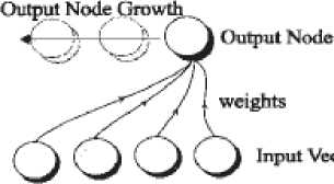
Figure I The Architecture of K-FLANN

KFLANN architecture consists of a single input layer that integrates the source of the patterns. The output layer grows dynamically as new classes are formed during the clustering phase. The weight connections between the input node and output node are the direct mapping of each element of input vectors.

• B.    Neural Network Input Parameters1)    Vigilance (ρ)

The Vigilance (ρ) is a parameter that originated from [18].It was designed as a means to influence the matching degree between the current exemplar and long term memory trace. The higher the ρ value, the stricter the match, while for a smaller ρ value, a more relaxed matching criteria is set .The ρ value in the K-FLANN is similar and it is used to determine the number of the attributes in the current exemplar that is similar to the selected output node. For example, if a pattern consists of 12 attributes and a clustering criterion was set such that a similarity of 6 attributes was needed for consideration into the same cluster, then the ρ should be held at 6/12=0.5.he Vigilance is calculated by ' Eq. (1)’ p = p;

Where ‘p’ is the total number of features and f is the number of features required to be classified in the same cluster. So the normalized value lies in between 0.5 to 1. If the vigilance value is high more number of clusters were formed than when it was s set lower.

• 2)    Tolerance (δ)

The tolerance setting of the exemplar attributes is the measurement of attributes dispersion, and thus computation is performed for every feature of the training exemplar at the initial stage. Tolerance setting (δ) for each feature is done by using binary search approach. This approach yielded good results, is the gradual determination of tolerance values based on the maximum and minimum differences in the attribute values.

Algorithm:

i)     Initially

• ii)    While number of clusters formed is not appropriate

• a)    Run standard KFLANN without step 8 based on Current δ i.

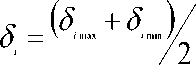
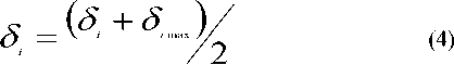
• b)    If number of clusters is less than expected

  5 =

  
  
  
  
  
  
  

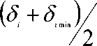
Else

If number of clusters is more than expected

End while

δ i. - Tolerance value for attribute i.

δ imin - Minimum difference in attribute values for attribute i. This is the difference between the smallest and the second smallest values of the attribute.

δ imax - Maximum difference in attribute values for attribute i . This is the difference between the smallest and largest values of the attribute.

• 3)    K-FLANN Algorithm

Step 1 Initialize the network parameters

Step 2 Present the pattern to the input layer. If there is no output node, GOTO step 6

Step 3 Determine all possible matches output node using

'Eq. (5)’.

У Dк-(w -x)2]

—------------------> p            ⁽⁵⁾

n

Step 4 Determine the winner from all matches output nodes using ' Eq. (6)’

Winner =

Step 5 Match node is found. Assign the pattern to the match output node. GOTO Step 2

Step 6 Create new output node. Perform direct mapping of the input vector into weight vectors.

Step 7 If a single epoch is complete, compute clusters centroid. If centroid points of all clusters unchanged, terminate.

Else

GO TO Step 2.

Step 8 Find closest pattern to the centroid and reshuffle it to the top of the dataset list, GOTO Step 2.

Where ρ is the Vigilance Value, δi is the tolerance for ith feature of the input space, W ij used to denote the weight connection of jth output to the  ith input, Xi represent the ith feature, D[a] = 1 if a > 0,Otherwise D[a] = 0.

value is 1, then it indicates more strict match means that all the features are participated in the clustering. If ρ value is less than 1 indicates that only some of the features contributed in getting correct number of clusters. The data sets used in this work are obtained from the site [16].

A. Exhaustive Search

Exhaustive search is performed on data sets which are having number of features <20. As stated above, optimal feature subset selection is possible only by using this method. (The mark (√) indicates the presence of feature. Rho value is set to 1 means that stricter match.

• 1)    Iris data set.

Iris data set contains 150 data patterns and 3 classes. It contains 4 features .They are

• 1  sepal length

• 2  sepal width,

• 3  petal length

• 4  Petal width.

The classes are Iris Setosa, Iris Versicolour, and Iris Virginica.

The best feature subsets selected among all (16 subsets) are shown below.

4) Modifications in the K-FLANN Algorithm:

Step 4 Determine the winner from all matched output nodes using the following criteria:

If same match is found

Winner= min     ( w..

L^ 0   ^j

^- xi ) ²

Else

Winner =

max

fs ^к - ⁽ w

^“

x) П

n

Table 1 features contribution for Iris data set

S.No.	1	2	3	4	No. of clusters	Error Rate (%)
1		√	√		3	4
2		√	√	√	3	4
3	√	√	√	√	3	4
4			√	√	3	4.666
5	√	√	√		3	4.666
6	√	√			3	5.333
7		√			3	7.333
8	√		√	√	3	7.333
9	√		√		3	8
10		√		√	3	9.333
11			√		3	9.333
12				√	3	23.333
13	√				3	40.666
14	√			√	1	44.666
15	√	√		√	9	66.666

V

V. Experimental Results

The clustering using modified KFLANN is controlled by vigilance (ρ).If more than one feature is present; there will be a chance of setting ρ value. If ρ

Table 1 was sorted based on error rate in ascending order so as to show the combinations achieving the minimum error rate at the top. The following observations can be made from this table.

1. The first three combinations have obtained the maximum accuracy of 96%

• 2.    Features 2 and 3 i.e. sepal width and Petal length are present in all the combinations (first 5 combinations).

• 3.    Without petal length in most combinations increases the error rate (%).

Better results are obtained for first 11 combinations out of total (15) yielding the accuracy is above 90%. With iris data set

• 2)    wine data set

• 1)    Alcohol

• 2)    Malic acid

• 3)    Ash

• 4)    Alcalinity of ash

• 5)    Magnesium

• 6)    Total phenols

• 7)    Flavanoids

• 8)    Nonflavanoid phenols

• 9)    Proanthocyanins

• 10)    Color intensity

• 11)    Hue

• 12) OD280/OD315 of diluted wines

• 13)    Proline

The best feature subsets selected among all (213 subsets) are shown below.

Table 2 Features Contribution for Wine data set

S.No

1

2

3

4

5

6

7

8

9

10

11

12

13

clusters

Error rate (%)

1

√

√

√

√

√

√

3

2.809

2

√

√

√

√

√

√

3

2.809

3

√

√

√

√

√

√

√

3

2.809

4

√

√

√

√

√

√

√

3

2.809

5

√

√

√

√

√

√

3

2.809

6

√

√

√

√

√

3

3.371

7

√

√

√

√

√

√

√

3

3.371

8

√

√

√

√

√

√

√

√

3

3.371

9

√

√

√

√

√

√

3

3.371

10

√

√

√

√

√

√

√

√

√

3

3.371

11

√

√

√

√

√

√

√

3

3.371

12

√

√

√

√

√

√

3

3.371

13

√

√

√

√

√

√

√

3

3.371

In the table shown above, the rows are sorted in ascending order. Only about 13 combinations are shown even good results were obtained for 100 s of combinations. For wine data set, the cutoff percentage of accuracy was taken as 96%.More feature combinations i.e. for 75 feature combinations out of 8192 combinations the maximum percentage of accuracy is (100-2.809= 97.19%) and minimum percentage of accuracy is (100-4.494=95.5%).By observing the frequencies of features, it was cleared that the features 1,7,10,11,12,13 have contributed more in clustering and achieved minimum error rate. For convenience only some results are shown whose percentage of error rate equal to greater than 96.50(%).

• 3)    New Thyroid Data Set

This data set contains 215 instances and 3 classes namely (normal, hyper, hypo).All five attributes are continuous attributes.

The best feature subsets selected among all (25 subsets) are shown below.

Table 3 Features Contribution for New Thyroid Data set

S.No	1	2	3	4	5	# of clusters	Error Rate (%)
1	√	√			√	6	11.63
2		√	√			3	12.55
3		√				3	13.95
4		√	√		√	3	14.41
5	√				√	3	14.41
6		√			√	3	14.88
7		√		√		3	15.81
8	√	√				3	15.81
9	√	√	√			3	15.81
10	√	√		√		3	19.06
11	√	√	√	√		3	19.53
12	√			√		3	22.33
13			√			3	22.79
14	√		√		√	7	22.79

For new thyroid data set, feature 2 contributes more because error rate is low when it is present (minimum is 11.63% and maximum is 19.53 and setting cutoff percentage of accuracy is 80%).The last three rows show that the performance of the algorithm is degraded if feature 2 is absent.

• B.    Heuristic Search

It is possible to reduce the search space by using heuristic search method. When the node is evaluated by K-FLANN, if child node has maximum error rate than current node error rate then the feature selection was stopped. Optimal feature subset selection is not possible with this method because the algorithm will always follow a single path at one level. The number of levels in the search tree are less than or equal to (d+1) where‘d’ is the total number of features in the data set.

The following table shows the feature subsets selected for the data sets used.

Table 4 Feature Subsets selected by Heuristic Search

Data Set	Feature Subsets in all levels	Error Rate (%)
Iris	3; 2,3; 2,3,4; 1,2,3,4 (All)	9.33; 7.33; 4; 4
Wine	10; 10 13; 10 12 13; 1 10 12 13; 1 6 10 12 13; 1 3 6 10 12 13; 1 3 4 6 10 12 13	30.8; 18.5; 8.42; 4.49; 3.37; 3.37; 3.37
New Thyroid	2; 2,3	13.95; 12.55

In the above table semicolon (;) indicates feature subset selected in respective level. For iris data set, in the third level itself the accuracy is 96% and when feature1 is added (last level), all the features contributed in clustering resulting same accuracy. For Wine data,7 (features are selected out of 13 which results an error rate 3.37%.For New Thyroid data set, two features contributed in clustering yielding the error rate 12.55%.

• C.    Comparison between Exhaustive Search and Heuristic Search

Table 5 Comparison between Exhaustive search and Heuristic search

S.No	Data Set	Exhaustive Search Best Solution (Minimum Error Rate (%)	Heuristic Search Best Solution (Minimum Error Rate (%)
1	Iris	4	4
2	Wine	2.809	3.37
3	New Thyroid	11.63	12.55

The above table shows the performance of two search algorithms. For iris data set, when Exhaustive search was used, the feature subsets participated in clustering to yield good results are 2 3; 2 3 4; 1 2 3 4 [from table 1]. But same result was obtained by heuristic search with 2 feature subsets (2 3; 2 3 4) [from table 4].For the New Thyroid data set, when Exhaustive search was used the features 1, 2, 4 are contributed [from table 3] in clustering results an error rate 11.63% but features 2 3 are selected by Heuristic search with error rate 12.55% [from table 4]. For wine data set, when Exhaustive search was used the attributes not present in the first 5 rows of the table 2 are 2,5,6.8,9 which results an error rate 2.8%[from table 2 ].With heuristic search features 10,12,13 are contributed more which results an error rate 3.37% [from table 4].

• VI. Conclusion

In this paper contribution of attributes in clustering multidimensional data using modified K-FLANN was discussed. The result of the modified K-FLANN i.e. how the data was partitioned depends on two parameters tolerance (δ) and vigilance (ρ). Tolerance for all the features was computed by Max-min method and was fixed initially. With the fixed tolerance and with the possible vigilance value (based on features match) the modified.

K-FLANN algorithm was run until stable centroids are formed. So using the vigilance parameter, it is possible to show the features contribution in the output. Both the methods used in this paper i.e. Exhaustive search and heuristic search are expensive as the number of attributes increases. The exhaustive search is performed for wine data set also with all 8191 possible combinations of features because 13 features present in the data set. The algorithm runs very well even with large input. So the KFLANN algorithm was scalable. But it is possible to reduce the search space by heuristic method when compared to exhaustive search. But it was shown that, optimal results were possible only with exhaustive search when compared to heuristic search. So in future, optimization techniques can be applied to set input parameters of the neural network and to select feature subsets.