Development of the actual state principle for a physical system

Original article

The main idea of the approaches considered in this article is that the state variables used to describe a physical phenomenon can always be divided into two groups. The first group consists of the so-called measurable variables, the values of which can be directly measured using the necessary equipment. Such quantities include displacement, speed, temperature, etc. The second group represents unmeasured quantities; unlike the elements of the first group, the values of such variables cannot be obtained by direct measurement, but only indirectly using appropriate mathematical models. For example, stresses in a extended rod can be identified based on measured displacements and a mathematical model of an elastic rod. Such variables include stresses, impulses, heat flows,

etc. At the same time, the governing equations can be divided into three groups. The first group includes the laws of balance and continuity. Initial and boundary conditions form the second group. The governing equations can be presented in the third group. The first type of equations reflects the influence of the environment on the system under consideration. The second describes the fundamental physical laws and hypotheses about the continuity of the environment. The defining relationships from the third group connect measurable and unmeasurable unknowns and contain information about the internal properties of the phenomenon being studied.

In physics, it is assumed that some of the governing equations are weakened in generalized formulations. The essence of the method of integro-differential relations,

THE RESULTS OF THE SPECIALISTS’ AND SCIENTISTS’ RESEARCHES substantiated in the book [1], is that equations of the third type are considered in integral form, while the remaining equations must be exactly satisfied. For example, the initial-boundary value problem can be reduced to minimizing a non-negative functional with respect to all admissible variables. This modification was the starting point to develop the modern numerical methods for analyzing states, assessing the quality of solutions, and optimizing processes in the dynamics of solids. Note that this method is also applicable to other boundary and initial-boundary value problems of mathematical physics [3, 4].

MATHEMATICAL MODELING IN ELASTICITYTHEORY

and from the boundary conditions

u = ii[(xj), хе 「 1 ，

О • n = % ( X J), X £ 「 2

(2.6)

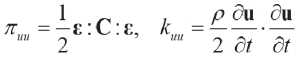
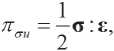
Let us present a more detailed consideration of the constitutive equations by groups using the example of the problem of linear elasticity. First, all constitutive equations in elasticity theory are composed of measurable variables u ( t,x ) – the displacement vector, which depends on time t and the spatial coordinate x , as well as unmeasurable variables σ ( t,x ) – the stress tensor (second-rank tensor) and p ( t,x ) – the momentum density vector. Second, the variables are chosen so that all energies, as quadratic forms, are written as direct products of the corresponding variables. The potential energy density π_σu has the form

and also special geometric constraints and also special geometric constraints (2.3). Here u ₁( x,t ) and q ₂( x,t ) are given boundary functions, n is the vector of the outer normal to the boundary of the body and t₀ is the initial moment of time. These relations are determined by external conditions.

The third group includes equations of state that relate measurable and unmeasurable unknowns.

p-Q^~ = 0, G-C ： € = 0.              (2.7)

Note that only these equations contain information about the internal properties of the object under study.

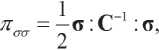
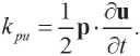
Using relations (2.7), (2.1) and (2.2) it is possible to calculate the densities of potential and kinetic energies expressed relative to only measurable or unmeasurable variables. The measured unknown quantities can be represented as

and accordingly immeasurable

(2.1)

(2.8)

(2.9)

and the kinetic energy density k_pu can be represented as

(2.2)

ε – the strain tensor can be represented as

(2.3)

a colon denotes the double tensor convolution operation, and a single dot denotes a simple scalar product.

The first group includes the equations of dynamic equilibrium (balance equation)

Note that calculating energies of this type is, generally speaking, not a trivial task. For example, if the problem is solved within the framework of nonlinear elasticity theory.

The initial-boundary value problem, modified in accordance with the variational approach [1], can be, for example, reduced to minimizing a quadratic nonnegative (energy) functional with respect to all admissible variables.

Let us compose a quadratic form

(2.4)

(2.10)

This equation relates only unmeasured variables, namely, stresses σ and impulses p . However, the properties of the medium are not included in this relationship. These equations reflect the laws of balance and continuity.

The second group consists of the initial

In the book [1] it is shown that the energy functional Φ composed using this form (2.10) is always non-negative

;…『陪J    (2.5)

① (u,g)= J e(u”)JQ 山 2 0, (2.11)

if the displacement u and stress σ fields strictly satisfy the relations (2.3)–(2.6). Here Ω× Τ is the space-time domain on which the problem is solved. The essence of this functional is that it consists of six different energies. Three of them constitute a quadratic relation, following from the

THE RESULTS OF THE SPECIALISTS’ AND SCIENTISTS’ RESEARCHES state equation, connecting stresses and deformations, and the other three follow from the relation with respect to the momentum and velocities of the body points. Using the notations introduced by (2.1), (2.2), (2.8) and (2.9), inequality (2.11) can be represented as

①(u,，)= П„„+ Пстст - 2Пот, + К“, + Kg - 2Km 2 О, п„„ = J 勾/Qd/, Пстст = J %“dQd/, Г!。,，= J jdQdt, CxT                   CxT                   CxT

(2.12)

CxT                  CxT                   CxT

In [1], a variational problem is studied in detail, in which the minimum of the functional (2.11) is determined under constraints (2.3)–(2.6), and it is proved that such a formulation is a variational principle. It can be shown that if all relations (2.3)–(2.7) are strictly satisfied, then the value of the functional (2.11) is identically equal to zero.

. (2.13)

Usually, when solving the problem numerically, it is not possible to strictly satisfy condition (2.13). Such a discrepancy can be caused by a number of reasons. Firstly, the chosen numerical solution method does not allow finding an exact solution. Secondly, within the framework of the formulated problem, not all of the relations (2.3)– (2.7) can be strictly satisfied. This circumstance indicates some imperfection of the mathematical model. However, this energy approach allows us to estimate the accuracy of the numerical solution. For these purposes, various relative estimates of the quality of the approximate solution can be made. For example, the ratio of the functional Φ to the value of the potential energy Πσσ

(2.14)

can be successfully applied to evaluate not only the accuracy of the numerical solution, but also the imperfection of the mathematical model used.

TWO-DIMENSIONAL PROBLEM OF ELASTICITY THEORY (STATIC CASE)

As an example, consider the plane bending of a rectangular elastic plate (see Fig. 1) occupying the following region Ω = { x ∈ (0, x ₀), y ∈ (0, y ₀)}. It is assumed that the homogeneous isotropic plate is loaded with some shear stress q ( y ) distributed along the edge Γ₁ with coordinate x = x₀ . The body is clamped along the edge Γ₃, where x = 0 . The others edges Γ₂ and Γ₄ of the plates are free from loads. Thus, the boundary conditions have the form

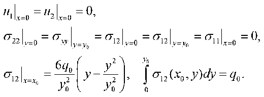
(3.1)

The desired solution u and σ is approximated by polynomials given by the formulas

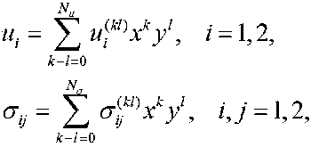
where u_i^(kl) and σ_ij^(kl)

(3.2)

are the unknown coefficients of the displacements and stresses components, respectively,

N_u and N_σ are the degrees of the complete polynomial approximations u_i and σ _ij. It is believed that the degrees of the polynomials for displacements and stresses are related N = N +1.

uσ

Since the region occupied by the body is convex, the homogeneous equation for the displacements and the polynomial constraints on the stresses (3.2) together with the equilibrium condition (2.4) can be exactly satisfied without degeneracy of the approximations for the displacements and stresses in after an appropriate choice of the polynomials degrees N_u and N_σ .

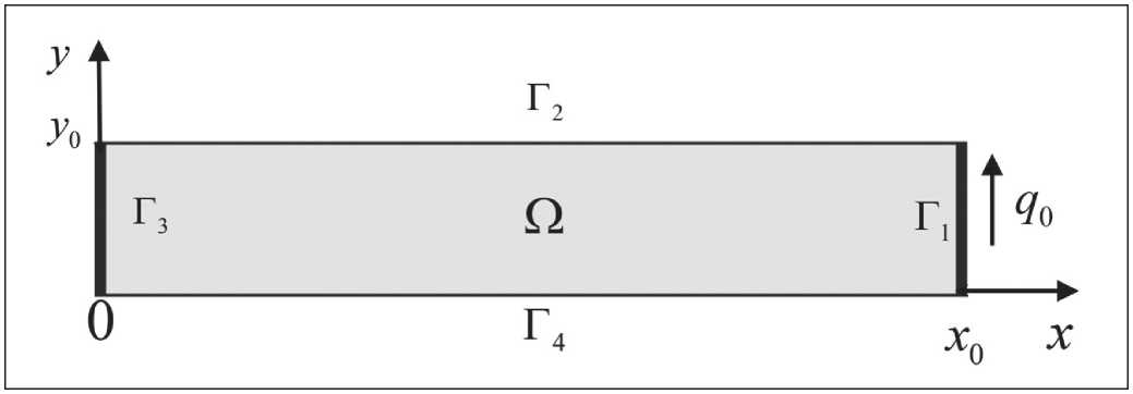
Fig. 1. Rectangular elastic plate

THE RESULTS OF THE SPECIALISTS’ AND SCIENTISTS’ RESEARCHES

Taking into account (3.2), two-dimensional equilibrium equations can be represented by componentwise

(3.3)

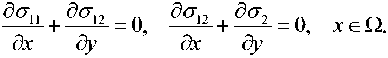
From equations (3.2) and (3.3). it follows that the coefficients σ _ij^(kl) must obey linear relations

(к + l)cr 俨丿)+ (/ + 1) 吊丁 D = О,

(左+ 1 ) 讨罗 J ) + ( /+1 ) ну+l ) = 0,

0<^ + /<^-1,                 (3.4)

The boundary conditions (3.2) are satisfied in a similar manner.

After satisfying the equilibrium equations (3.4) and the boundary conditions, the following unconstrained minimization problem arises: find a vector a ^* ∈ R^N that minimizes the following functional

^^("j ， 0 曾 ) 一 i 1"" + ' 丄 57 2] ]<7?/ ^ ^^9 '   (3.5)

Since a static problem are consideried, kinetic energies do not enter into (3.5). Here a ∈ R^N is a vector of design parameters consisting of N independent coefficients u_i^(kl) and σ_ij^(kl) , which remain in equations (3.4) and (3.2) after solving all equilibrium equations and boundary conditions.

After integration over the domain Ω, problem (3.5) is reduced to minimizing the corresponding quadratic form

Ф(а) = а^тКа - 2(F)^T а —吗? .         (3.6)

Here K ∈ R^N×N is a symmetric and positive definite matrix and F ∈ R^N is a vector determined by the boundary surface forces. The vector a that minimizes the corresponding functionals is found as a solution to the linear system of equations:

Ka = F.

(3.7)

The following dimensionless geometric and material parameters were chosen: plate length x ₀ = 1 and height y ₀ = 1, Young’s modulus E = 100 and Poisson’s ratio ν = 0.3, external force q ₀=1. The calculations were performed with various polynomial approximations of degree N _σ = 8,…,16.

The elastic energies Π uu , Π uσ , and Π_σσ are shown in Fig. 2. As can be seen from this figure, the approximate value Π_uu (solid line) of the elastic energy decreases monotonically with increasing order N _σ. In contrast, the values of the energies Π_uσ and Π_σσ (dotted and dash-dotted curves, respectively) increase monotonically as the number N _σ increases. It can be concluded that the exact value of the elastic energy lies between the extreme lines.

This approach allows one to analyze explicitly the distribution of local errors. For this purpose, the energy residual density φ /Π_σσ from formula (2.10) can be used. As can be seen in Fig. 3, for the problem under consideration with N _σ = 16, this function has maximum values at the same points where the elastic energy density is concentrated. The function φ indicating the features of the solution can be used to refine and adapt the mesh in FEM procedures to improve the quality of the approximate solution.

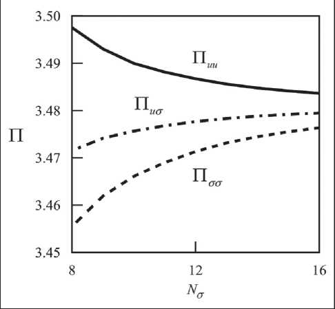
Fig. 2. Elastic energies Π_uu, Π_uσ, and Π_σσ as functions of the number of degrees of freedom N

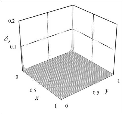
Fig. 3. Distribution of energy error φ over the region Ω

THE RESULTS OF THE SPECIALISTS’ AND SCIENTISTS’ RESEARCHES

MATHEMATICAL MODELING IN FLUID THEORY

Supplying water to buildings under sufficient pressure is an important problem for modern life. Reliable control of numerous piping systems to consumers is required for comfortable and safe supply. Typical piping systems consist of several widely distributed elements, such as long pipe sections transporting water using several control pumps. Adequate mathematical models of piping dynamics, defined in terms of partial differential equations (PDE), must take into account distributed system characteristics, such as the compressibility of the medium and variations in fluid pressure and mass flow [5].

Let us consider a pipeline element consisting of a long straight section of pipe with transported liquid supplied by a control pump. One-dimensional motions of compressible viscous liquid inside a rigid cylindrical pipe are described in a Cartesian coordinate system with an axis directed along the central line of the pipeline with the origin at its left end cross-section.

It is assumed that the average fluid pressure in any section of the pipe 歹 =P o +p(%X ) , as well as the mass flow rate of the fluid through this section q = %+q 化 x) , do not deviate too much from their nominal values p ° > 0 and q₀. In what follows, all system models and control procedures are derived in terms of excess pressure p and mass flow rate q . In the compressible fluid model, pressure is expressed as a linear function of excess bulk density according to

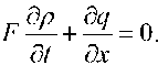
The equilibrium equation for the flow is defined as

《■+卓 +«x,/p) = °, ot ox

(4.5)

Where r is the linear density of the fluid resistance forces in combination with external loads, such as gravity.

The boundary conditions are given by the expression and                . (4.6)

Finally, the initial conditions can be written as and                 . (4.7)

The variables u⁰ and u ¹ are either given functions of time t or unknown control inputs.

By analogy with the methodology described in the previous paragraph, two types of variables can be distinguished. The measured variables include the effective displacement function w(t,x) , and the unmeasured variables include the mass flow function q(t,x) and the fluid pressure p(t,x) . All equations given in this paragraph are divided into three groups. The first group includes the fluid flow equilibrium equations (4.5) and the continuity equation (4.2). The second group includes the boundary (4.6) and initial (4.7) conditions. The third group includes the equations of state (4.4) and (4.1). Note that equation (4.1) was used to exclude density.

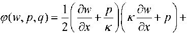
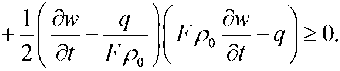
Let us construct a quadratic form using the equations from (4.4),

,

(4.1)

where p о = const is the nominal density of the liquid, and к = const is the bulk modulus of elasticity.

The nominal average pressure in the pipeline system must be high enough to ensure the continuity of the liquid medium in accordance with

(4.8)

(4.2)

Here F is the cross-sectional area of the pipe.

Let us introduce an auxiliary function of effective displacements w(t,x) that determines the distribution of excess bulk density p(t,x) and mass flow q(t,x) through

The positive definiteness of the form (4.8) follows directly from the positivity of the coefficients к > 0 and Fp о > 0.

Integrating (4.8) over the length of the pipe and the duration of the time interval, we obtain

. (4.9)

Ow ,    ” 碗 and              .

(4.3)

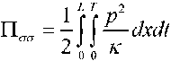
Here the notations for potential energies are introduced.

It can be shown that the continuity condition is identically satisfied after substituting definition (4.3) for the volume density into (4.2). Eliminating the function p , the defining relations (4.1) and (4.3) can be represented as

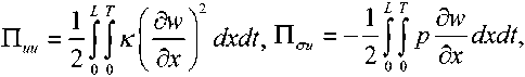
and                   .

(4.4)

(4.10)

THE RESULTS OF THE SPECIALISTS’ AND SCIENTISTS’ RESEARCHES

To develop an optimal control law, we consider a polynomial input control as

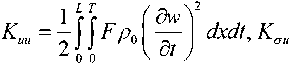
and for kinetic energies

中陪м

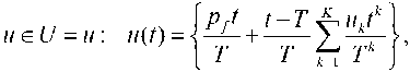
〃 (0) = 0 ，〃 (T) = p_f .

K^=^\\^rdxdt-

厶 0 0 丄 к0

(4.11)

(5.4)

It can be shown that if all relations (4.1)–(4.7) are strictly satisfied, then the value of the functional (4.9) is identically equal to zero.

① (w, 。)三 0. (4.12)

This energy approach always allows us to estimate the imperfection of the constructed numerical solution. As in the previous paragraph, various relative quality estimates of the approximate solution can be constructed for these purposes. For example, we can limit ourselves, as in the previous case, to estimate (2.14).

OPTIMAL PRESSURE CONTROL

The problem of optimal pressure control is to find a control pressure as an input u^*(t) to the system from a given set of controls U that transfers the pipeline system from the initial state (4.7) to the final equilibrium state with the desired pressure and mass flow distribution along the pipe in a fixed time T according to

P ( T,x) = Pr ( x), q(T,x)^O.

(5.1)

Here p_T is the stationary distribution of the final pressure of the liquid. In this case, the objective function J ₀[ u ], which describes the effective residual energy of the entire system, must be minimized:

After solving the initial boundary value problem described by the functional (4.9), using the method discussed in detail in Section 2, the solution is found for uncertain components of the vector u = { u₁,…,u_k } of control parameters. The resulting vector functions w ˜(t, u ) and q ˜(t, u ) are used to minimize the modified objective function

4 (u) f min, 4 二 ％ (u) + ^ Ф(и), (5.5)

where the additive term with a dimensionless weighting coefficient γ affects the numerical value of the optimal solution conditionality. The tilde symbol in (5.5) means that the corresponding functionals are expressed through the solutions w ˜, q ˜ after substituting them for the optimal values. The vector u ^*, obtained as a result of finding the optimal control function u ^*(t) = u (t, u ^*), is used for subsequent numerical simulations.

To demonstrate the efficiency of the optimization algorithm, two controlled processes in a pipeline system are considered. The first process corresponds to the flow of an ideal fluid in a homogeneous sealed pipe without resistance ( κ ₀ = κ ₁ = 0). In the second process, the fluid flow is characterized by a constant and viscous resistance with system coefficients ( κ ₀ = κ ₁ = 1). The control parameters T = 4, p_f = 1, K = 9, γ = 10, are used for all examples in this section.

The time diagram of the optimal pressure control u^*(t) is shown in Fig. 4 for both processes. The control laws for

4 [и] f mm, 4 = E(T\ E(T) = [ 〃亿 x)dx, 〃 = ( ?_/ ；) +q , Рт^p_f^+K^~^x\

〃 (0) = 0, 〃 (T) = Pf.                         (5.2)

All relations are reduced to dimensionless form by substituting variables in accordance with

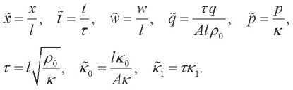
(5.3)

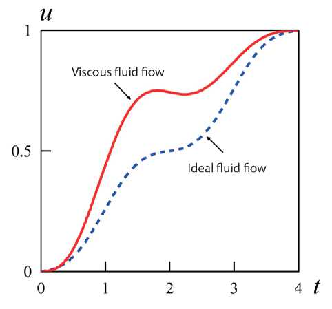
Fig. 4. Optimum boundary pressure

In what follows, the tilde signs are omitted in all equations.

THE RESULTS OF THE SPECIALISTS’ AND SCIENTISTS’ RESEARCHES

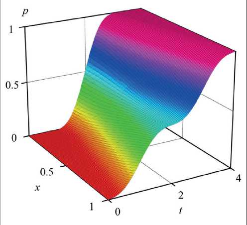
Fig. 5. Pressure distribution for an ideal fluid flow

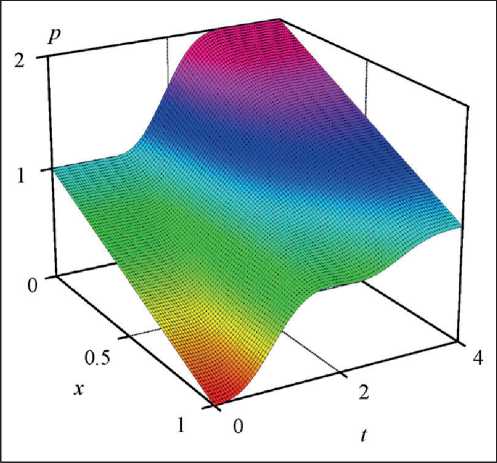
Fig. 6. Pressure distribution for a viscous fluid flow

the ideal and viscous fluids are shown in this figure by the dotted and solid curves, respectively. It is seen that the optimal pressure control is higher if the resistance along the pipe is taken into account. In addition, the monotonic nature of the control function is violated in the case of a viscous fluid.

Figure 5 and Figure 6 show the fluid pressure distributions for both ideal and viscous fluids in space and time. Note that the proposed control strategy allows us to transfer systems from their initial states to a close neighborhood of specified final pressure distributions p _τ(x) in such a way that undesirable oscillations are prevented.

The value of the cost function defined in (5.2) is J ₀ = 9.6 • 10^–8 for an ideal fluid. The relative integral error introduced in (2.14) is quite small for this approximation: δ_σ = 1.6 • 10^–9. For the model with viscous drag, these values are significantly smaller than those obtained for an ideal fluid and are equal to J ₀ = 3.9 • 10^–10 and δ_σ = 7.1 • 10^–11, respectively. This means that viscosity in a linear fluid model can be a valuable factor in improving the quality of approximate solutions. Moreover, it helps to reduce the intensity of residual oscillations.

ENERGY PRINCIPLE IN THE HEAT TRANSFER PROBLEM

Let us consider the process of heat transfer in two spatial coordinates in a rectangular plate with dimensions a and b . The law of heat flux transfer (Fourier’s law) relates the heat flux density vector

9 = [% ， (y ， zJ),/(y,z/)] =

=[風豆 (У, z J), 朋厶 (У, z/)] (6.1)

and temperature gradient:

_п дө _ 。 se 八

%+X 百=%+'可=°

9z + 4 大~ = 9z + 4= = °

{У, z, /}gQx{0, T},

Q = (-q / 2, о / 2) X (-6 / 2, 方 / 2).

(6.2)

Here temperature is denoted as θ(y,z,t) and λ is the thermal conductivity coefficient. In order to use the methodology described in the previous paragraphs, new variables q_y = q ˜ _y , q_z = q ˜ _z, θ = 色 θ , are introduced into these equations. As can be seen, such a replacement does not change the form of equations (6.2). Here θ_a is the ambient temperature.

The first law of thermodynamics leads to реp( + 2+ .吟""(义2,。; °,  (6.3)

ot oy OZ п where ρ is the bulk density of the plate material, cp is the specific heat capacity, α is the convective heat transfer coefficient, and h is the plate thickness. The function µ(y,z,t) represents both distributed control and external disturbances.

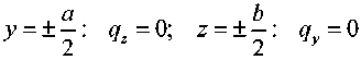
In terms of heat flux densities q_y and q_z boundary conditions are given as

%,(y,±b/2,/) = 0, q_:(+a/2,x, 0 = 0. (6.4)

To complete the formulation of the initial boundary value problem, we define the initial temperature distribution

THE RESULTS OF THE SPECIALISTS’ AND SCIENTISTS’ RESEARCHES

e ( y,z, o ) = 〃 o,z ) .

(6.5)

In complete analogy with the case of linear elasticity considered in the previous section, the heat transfer equations (6.2) – (6.5) can be combined into three groups by introducing a new function r_q in such a way that equation (6.3) takes the form

噥 +% ( y ， z,/) = o,               (6.6)

where

分+勺 3 一勺 6- 〃 =分+勺心 .         (6.7)

Here, for convenience, new parameters κ ₁ = ρc_{p ,} κ ₂ = 2α/h = h , and r_θ = ∂ θ/ ∂ t - κ ₂ θ/κ ₁ µ/κ₁ , are introduced. Explicit indication of the initial and boundary conditions for r_q is not required, since they are already completely determined by equations (6.4) and (6.5).

Thus, equation (6.6) is included in the first group of equations. This is an analogue of the equilibrium equation (2.4). The boundary (6.4) and initial (6.5) conditions belong to the second group. Relations (6.2) and (6.7) constitute the third group of equations, and only these relations contain information about the properties of the material.

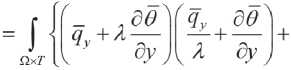
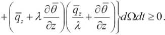
By analogy with the initial-boundary value problem (2.4)–(2.7), it is important to consider the quadratic values of the defining relations (6.2) and (6.7). The discrepancy in the assignment of potential (thermal) energy, which follows from (6.7), can be represented in the form

% =町 .-2 匕 + % =

CxT          I *1 丿

Then, if all relations (6.2)–(6.7) are strictly satisfied, then the value of the functional (6.10) is identically equal to zero.

①（仇外三 0

(6.11)

As in the previous cases, this approach allows us to estimate the imperfection of the constructed numerical solution. For these purposes, we can construct various relative estimates of the quality of the approximate solution. For example, we can limit ourselves, as in the previous case, to estimate (2.14).

TWO-DIMENSIONAL HEAT TRANSFER PROBLEM

Consider a rectangular metal plate, shown in Fig. 7. There is a set of geometric and physical parameters of the system that are used in modeling. The dimensions of the plate are shown in this figure.

The physical parameters of the plate are as follows:

2 = 110Bt-m4-K^, " = 2700кг・м-з, ср =896Дж-кгч-Ю1, а = 60Вт-м"2-К1. (7.1)

The parameters of this model were determined in a series of experiments.

In terms of heat flux density, the boundary conditions are given by the expression

.

(7.2)

It is assumed that all sides of the plate are adiabatically insulated. Thermal action (control) on the plate is carried out using Peltier elements in combination with cooling devices (colored areas in the figure). Note that this type of control action can be taken into account by the function µ(y,z,t) in equation (6.3). If µ > 0, then this is a heating process. If µ < 0 – cooling.

From relation (6.2) one can formulate the discrepancy in the assignment of kinetic energy (heat flow).

① K=K“ 「 2Kg+K“

Thus, from (6.8) and (6.9) it follows

①(仇 4)= ① /+ ① K=n“, ， +IIg

-2Псти+^,+^-2^от>0.

(6.10)

(6.9)

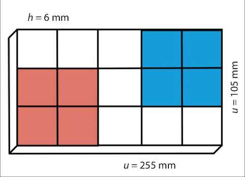
Fig. 7. Schematic diagram of the experimental setup

THE RESULTS OF THE SPECIALISTS’ AND SCIENTISTS’ RESEARCHES

The two control inputs are considered to be located on the colored parts of the plate. The lower part of the plate corresponds to the place where the plate is heated by the Peltier element with intensity 〃 [ (y,z,t) = 60 W/(abh) . The upper part of the plate is cooled with 4 2 (y,z,t)= 30 W/(abh) .

To take into account the discontinuous control function "(y,z,t) , a finite element scheme has been developed, shown in Fig. 8, based on a four-node quadrangular element. The interelement conditions (continuity) on each adjacent element have the form

. (7.3)

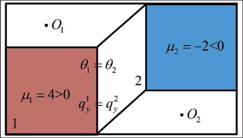
Fig. 8 Finite element mesh and interelement conditions

Polynomial approximations of the unknown functions of temperature and heat flux are given for each element in the following form

N

e = tf〉(t)yS,

* = 24 了(?)炉" к+1

^+l

.                                  (7.4)

A+l

Satisfaction of boundary conditions (7.2) using approximation (7.4) makes it possible to construct a system of ordinary differential equations for the time-dependent functions defined in equation (7.2). To construct a sequential differential problem, it is necessary to take into account the initial conditions (6.5).

The effectiveness of the proposed approach is illustrated in Fig. 9, which shows the temperature profiles. These time-dependent functions are calculated at points 0 1 and O 2 (shown in Fig. 8) and are represented by red and blue lines, respectively.

The increase in the accuracy of numerical solutions with an increase in the degree of the approximation polynomial is shown in Fig. 10 as an example of the change in the relative error 8 ° given in (2.14) and expressed as a percentage.

GENERALIZING PRINCIPLE

Any physical system is described by measurable and unmeasurable variables that satisfy boundary and initial conditions, as well as equilibrium equations, and are related to each other by governing equations.

Potential and kinetic energies in a system can be expressed in terms of measurable variables Π_u( u ), T_u( u ), unmeasurable quantities Π_σ( u ), T_σ( u ), and mixed energies Π_uσ( u,σ ), T_uσ ( u,σ ). Then the true state of the physical system is achieved when the linear energy relation is strictly satisfied

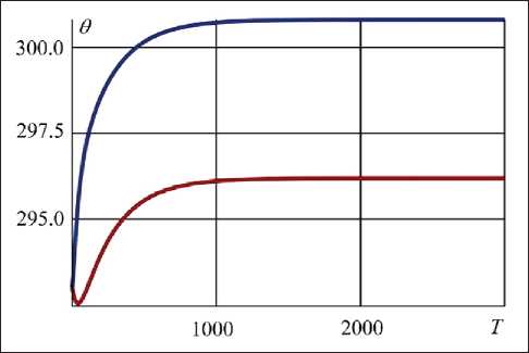
Fig. 9 Temperature profiles at points O₁ (upper curve) and O₂ (lower curve)

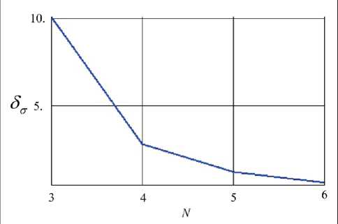
Fig. 10. Relative error δ_σ with respect to the degree of approximation N

. (8.1)

If the value of the functional (8.1) is not equal to zero, then the relative assessment of the accuracy of the approximate solution of the physical problem is equal to:

.

(8.2)

THE RESULTS OF THE SPECIALISTS’ AND SCIENTISTS’ RESEARCHES