Diagnostic Path-Oriented Test Data Generation by Hyper Cuboids

Author: Shahram Moadab, Mohsen Falah Rad
Journal: International Journal of Information Engineering and Electronic Business(IJIEEB) @ijieeb
Article in issue: 6 vol.6, 2014.
Free access
One of the ways of test data generation is using the path-oriented (path-wise) test data generator. This generator takes the program code and test adequacy criteria as input and generates the test data in order to satisfy the adequacy criteria. One of the problems of this generator in test data generation is the lack of attention to generating the diagnostic test data. In this paper a new approach has been proposed for path-oriented test data generation and by utilizing it, test data is generated automatically realizing the goal of discovering more important errors in the least amount of time. Since that some of the instructions of any programming language are more error-prone, so the paths that contain these instructions are selected for perform test data generation process. Then, the input domains of these paths variables are divided by a divide-and-conquer algorithm to the subdomains. A set of different subdomains is called hypercuboids, and test data will be generated by these hypercuboids. We apply our method in some programs, and compare it with some previous methods. Experimental results show proposed approach outperforms same previous approaches.
Diagnostics, Test Data Generation, Test coverage of code, Error-Prone Path, Symbolic execution
Short address: https://sciup.org/15013308
IDR: 15013308
Text of the scientific article Diagnostic Path-Oriented Test Data Generation by Hyper Cuboids
Published Online December 2014 in MECS DOI: 10.5815/ijieeb.2014.06.01
Since the most important step of designing of a test case is the test data generation [1], some references such as [2, 3] have assumed it equivalent to the test data generation. Test data generation, is done by the different methods such as genetic algorithm [4, 5, 6], randomly [7, 8, 9], etc. The test data generators are divided into categories of random generator, data specification generator, and path-oriented generator [10, 11].
The most powerful test data generator is the path-oriented one [12]. Generating of path-oriented test data which is also known as the path testing, is one of the most famous white-box testing techniques. This test is done in three basic steps including the selection of some paths, test data generation, and comparing the output which obtained from generating test data with the expected output. The purpose of the test data generation step is finding inputs that lead to the traverse of the selected path. Finding an exact solution set to complete solving a path constraints is NP-hard [13, 14]. Hence, the test data generation, is considered a major challenge in path testing.
Many previous works [15, 16, 17, 18] have tried to test data generation tools in order to automate this process. Dunwei Gong et al. [19] suggested an approach that has concentrated on the problems related to test data generation for many paths coverage, and has provided an evolutionary method for generating test data for many paths coverage that is based on grouping. Initially, target paths based on their similarities are divided into several groups, and each of these groups, converts a suboptimization problem into several simpler suboptimization problems; finally, the sub-optimization problem are facilitated with the test data generation process.
Lizhi Cai [20] proposed a business process test scenario generation that is according to the combination of test cases. In this method the test cases have been modeled in the form of TCN (Test Cases Nets) and a CPN (Colored Petri Nets). By combining of the existing TCN, the BPSN (Business Process Scenario Net) is created. Test scenario generation techniques were discussed for basis path testing and for a business process based on BPSN.
Arnaud Gotlieb and Matthieu Petit [21] by using a divide-and-conquer algorithm have generated random and uniform test data throughout the allowable area. In this method, generating test data is based on two basic concepts: constraint propagation and constraint refutation. The constraint propagation process, will pruned the domain of all constraints of a path from their inconsistent values, and also the constraint refutation process removes some part of the non-allowable area. Finally, test data are generated from remained area.
Ruilian Zhao and Yuandong Huang [22] have proposed a method in order to automatic path-oriented random test data generation, which is based on double constraint propagation. This approach reduces a path domain of program by splitting an input variable domain. This removes a wide domain of non-allowable area. Therefore, a few number of generated test data of this method will be rejected.
As a result, the proposed approach with the detection of more errors in less time has taken an important step to improve the testing process. Our approach was implemented by Turbo C++ 4.5 using the random function for random generation and was evaluated on several C and C++ programs. These experiments show that the error detection rate (EDR) and the error detection speed (EDS) ranges from 7.2 to 2804 times and from 4.8 to 228 times respectively, more than the same previous approaches.
In Section 2 we illustrate concepts and important terms of test data generation. In Section 3 a new approach is presented to generate path-oriented test data. Section 4 identify two criteria and contains the experimental results obtained from our implementation. In Sections 5 and 6, we respectively discuss the threats to validity and present the conclusion and proposed cases for future works.
-
II. Basic Concepts
-
2.1. Control Flow Graph
-
2.2. Test Adequacy Criteria
Path-oriented test data generation is based on fundamental and important concepts that will be described as follows.
The Control Flow Graph (CFG) in a program is a connected oriented graph which consists of a collection of vertices, including edges that each of them indicative a branch between two basic blocks and two distinct nodes, that each node indicative a basic block; which e and s represent the entry and exit nodes, respectively. Drawing a CFG has its own rules. If we have the function Foo as Fig. 1, then the CFG for this function can be depicted by Fig. 2.
After CFG construction, some paths of it should be selected for testing. Since the selection and traversing of the all existing paths is not practically possible, the selection of more appropriate path set is too important. If the number of selected paths be more, it is clear that more resources, effort, time, and costs will be required to generate the test data; instead, more errors will be discovered. Also, an important challenge in this step is selection of the path that will lead to the detection of more errors than the path that contains lower errors. In this regard, researchers have introduced the following void Foo(ush x, ush y){ if (x > y){ while (x ≥ 500)
x--;
cout << x;
} else{ while (x > y){
} …
}
Fig. 1. The Foo function
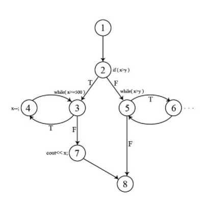
Fig. 2. CFG of function Foo criteria to select more appropriate path that are known as test adequacy criteria:
-
• Statement Coverage : In this criterion, that is the weakest among the white-box Testing criteria [2], each instruction is executed at least once. The advantage of this criterion is the ability to identify blocks of code that are not executed. The disadvantage of this criterion is that it is not able to detect many logical errors of the program.
-
• Branch Coverage (Decision Coverage) : In this criterion, in addition that the test cases are executed each instruction at least once, must execute all of its outputs at least once, against any decision [2, 24, 27, 28]. However this criterion satisfies the statement coverage criterion, but is not able to detect the errors of conditions in the combined decisions.
-
• Condition Coverage : In this criterion, in addition to each instruction is executed at least once, all possible composition of the conditions in a decision must also be executed [2, 24, 27]. The reason is that a decision may be a combination of several conditions. The advantage of this approach is the discovery of conditions errors inside the decisions and its disadvantage is the lack of attention to the different combinations of these conditions.
-
• Decision/Condition Coverage : In this criterion, in addition that each instruction is executed at least once, every decision and all the conditions within it are also executed at least once [2, 24]. The
advantage of this criterion is fixing two above criteria disadvantages and its disadvantage is the lack of considering all the different combinations of conditions.
-
• Multiple Condition Coverage : This criterion in addition to covering all of the above criteria, also considers all the different combinations of a decision conditions [2, 24]. The advantage of this method is fixing all of the above criteria disadvantages and its disadvantage is the lack of covering all paths of the program.
-
• All Path Coverage : This criterion runs all possible paths of the program at least once [24]. The advantage of this method is the cover the whole paths of program and its imperfections are possibility of execution the paths in excessive amounts and impossibility of traverse all program's paths.
-
• Simple Path Coverage : This criterion has executed all possible paths of the program at least once and does not run any part of the program in excessive amounts [24]. The advantage of this method is covering the entire paths of program and its disadvantage is that it is impractical; because traversing all paths of a program is impossible.
-
2.3. The Infeasible Path
-
2.4. Allowable Area
-
2.5. Hypercuboid
These criteria are listed respectively from weak to strong, and realization of a weaker criterion, is easier than the stronger criterion.
One of the major challenges is the possibility of existence the infeasible path. The infeasible path is the path that because of existence the contradictory conditions in it, is not traversable with any test data. For example, the path 1→2→5→6→5→8 of control flow graph is shown in Fig. 2 is a non-traversable path. Because the intersection of two contradictory conditions x≤y and x>y in this path is null.
The largest area that all generated test data in it, are lead to satisfy all the constraints of a specific path, is known as its allowable area. From the intersection of all constraints in one path, the allowable area is achieved. For example you can see the allowable area corresponding with the constraint set of path 1→2→3→7→8 from the Fig. 2 in Fig. 3.
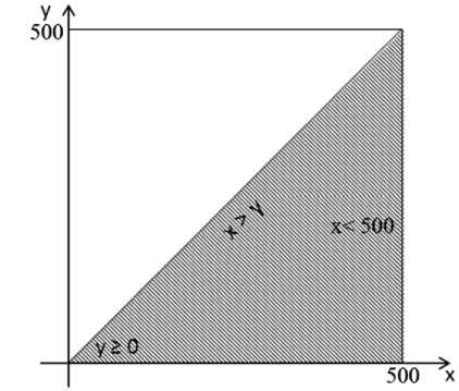
Fig. 3. A sample for displaying the allowable area
Each used variable in a program has a minimum and a maximum value. From intersection of intervals between the minimum and maximum values of the n variables in an n-dimensional space, an n-dimensional hyper cuboid is obtained. For example, consider the following variables and their related intervals:
x: 〈 1 ..20 〉 y: 〈 1 ..10 〉
z: 〈 1 ..30 〉
The 3-dimensional hyper cuboid as has shown in Fig. 4 is obtained from intervals intersection of these three variables. By selecting any arbitrary value from intervals of the variables in a hyper cuboid, a point will be obtained that certainly is inside the hyper cuboid. Therefore test data generation throughout of a hyper cuboid domain is easy because any of its points can be randomly selected by choosing its coordinates independently. For example, selecting any arbitrary value from intervals of the variables x, y and z is lead to generate a point that certainly will be inside the obtained hypercuboid from these variables.
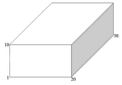
Fig. 4. A sample for displaying the hyper cuboid
-
III. The Proposed Approach
-
3.1. The Proposed Approach Procedure
-
3.1.1. CFG Construction
-
3.1.2. Labeling
The goal of our proposed approach is to generate diagnostic test data. Some of the test data are leading to the discovery of the errors and some of them are just traversing the desired path. Since a test is successful when it is able to detect an undiscovered error [2] it is essential to attend about generation of diagnostic test data instead of non-diagnostic one; while many of previous proposed approaches only have generated test data and haven't noticed whether it is diagnostic or not.
For the better understanding of the operation of the proposed approach, its procedure is shown in Fig. 5. In the figure, bubbles show the inputs and outputs of the program, rectangles show the process phases, and diamonds show the branches in the execution. The proposed approach is done in seven steps including CFG construction, labeling, path selection, symbolic execution of selected path, constraint propagation, consistent hyper cuboid extraction, and test data generation. Each one of the above seven-pace stages will be described separately.
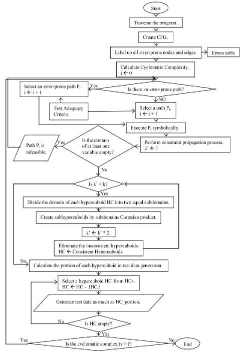
Fig. 5. The Proposed Approach Procedure
In the first step of the proposed approach, after traversing the program under test, the related CFG will be drawn (According to descriptions mentioned in section 2.1).
Table 1 is used for detecting an error-prone instruction. This table shows a list of the common errors in a C++ program [29]. In this table, the first column is the number of error, the second column is the name of that error, the third column is an example of a program with an error; the fourth column is the correct program of example in the third column, and the fifth and sixth columns, respectively, shows the output of a program with an error (third column) and the output of the correct program (fourth column). Since this table is contain error-prone instructions of C++ language but we can easily find the error-prone instructions of other programming language, and add to it. In this case, the other steps of proposed algorithm will be executed without any change.
-
3.1.3. Path Selection
Path is a finite sequence of edge-connected node in the CFG that starts from entry node. The number of selected paths in this step is equal to the calculated Cyclomatic complexity for the corresponding CFG. The number of Cyclomatic complexity is obtained by one of the following formula:
-
• The number of CFG areas
-
• E – N + 2
-
• d + 1
-
3.1.4. Symbolic Execution of Selected Path
-
3.1.5. Constraint Propagation
-
3.1.6. The Consistent Hypercuboid Extraction
In which E is the number of edges, N is the number of nodes and d is the number of predicate nodes in the CFG. Based on the McCabe’s proposed testing called basis path testing, the linearly independent paths can be select in this stage. A selected path will be linearly independent, if at least one non-traversal edge by previous selected paths existed in it. By definition, a set of linearly independent paths that their numbers are equal to the Cyclomatic complexity is called the basis path set. Since this basis path set is not unique, it is important to make more appropriate selection. Accordingly, at this stage, we will try to select the paths that are consist at least one labeled error-prone node. We called these paths the error-prone paths. For example, the path 1→2→3→7→8 of control flow graph is shown in Fig. 2 is an error-prone path. If
Table 1. Different Types Of Errors
To obtain the constraints of a path, the symbolic execution usually is used. In the symbolic execution, variables values are obtained without actual execution of the program and are based on the input variables and the constant values. It has been created a path constraint Φp for each execution path p, for example, a sequence of statements were executed by the program which indicating the input assignments that program executes along p. At this step, constraint set of the selected path, is obtained by symbolic execution of the previous step and is given as input to the next step.
Consequently, the minimum and maximum ranges for the variables x and y will be 100 ≤ x ≤ 400 and 100 ≤ y ≤ 300, respectively. During the pruning operation, if a variable range be empty, also the constraints intersection will be empty. This means that the path is non-traversable with any test data and so called an infeasible path [21]. In this case, algorithm returns to the path selection stage for selecting another path.
Each hyper cuboid by dividing each one of its subdomain to the two subdomains and Cartesian product of this subdomains, can be divided into the subhypercuboids. For example, consider the hyper cuboid shown in Fig. 4. If the domain of each one of its variables be divided into two parts, the following subdomains will be achieved.
x: 〈1 ..10〉, 〈11 ..20〉
y: 〈1 ..5〉, 〈6 ..10〉
z: 〈1 ..15〉, 〈16 ..30〉
With the Cartesian product of these subdomains eight hyper cuboids D1= ( x ϵ 1..10, y ϵ 1..5, z ϵ 1..15), D2= ( x ϵ 1..10, y ϵ 1..5, z ϵ 16..30), D3= ( x ϵ 1..10, y ϵ 6..10, z ϵ 1..15), D4= ( x ϵ 1..10, y ϵ 6..10, z ϵ 16..30), D5= ( x ϵ 11..20, y ϵ 1..5, z ϵ 1..15), D6= ( x ϵ 11..20, y ϵ 1..5, z ϵ 16..30), D7= ( x ϵ 11..20, y ϵ 6..10, z ϵ 1..15), D8= ( x ϵ 11..20, y ϵ 6..10, z ϵ 16..30) will be achieved, which you can see in Fig. 6. Each of the obtained subhypercuboids, also are a hyper cuboid. At this step, after the generation of subhypercuboids at each time, the inconsistent subhypercuboids will be eliminated by the consistency check algorithm. The remainder consistent subhypercuboids also are divided into 2n subhypercuboid that n is equal to the number of variables. Eliminating of the inconsistent subhypercuboids apply on the obtained subhypercuboid again.
This process continues until dividing the domain of each variable to the k subdomains. Value k is determined by the tester and based on the time constraints. Whatever the value of k is greater, more non-allowable area will be removed by eliminating the inconsistent subhypercuboids; instead, more time will be spent for subhypercuboids generation. Achievement the optimal value of k is difficult and is obtained experimentally. The reason of gradual division of domains instead of suddenly division is that with the gradual division in each step, a greater volume of the allowable area will be removed with the less number of using the consistency check algorithm. In many previous works such as [21], this value cannot be exceeded of a small amount (usually 4). Because due to using of the time consuming consistency check algorithm, with increase the amount of k, the running time of algorithm will be increased extremely. Our proposed consistency check algorithm fixes the above problem greatly. The method of this algorithm is that it checks all corners of a hyper cuboid. If none of these corners were able to satisfy the constraints of the constraint set, detects it as a possibly inconsistent hyper cuboid. The reason that we used the word "possibly" is that all corners of a hyper cuboid may be outside of the allowed area, but a part of hyper cuboid is within this area. The hyper cuboid D2 in Fig. 7 is like this. However this problem does not happen in most programs, and if occurrence will be included only a few of hyper cuboids. To improve this problem, we also generate a few random test data of possibly inconsistent hyper cuboid. If none of these generated random test data can satisfy the constraints, the proposed consistency check algorithm, eliminates the hyper cuboid. The number of generated random test data, is dependent on the time constraints of the project.
-
3.1.7. Test Data Generation
-
3.2. Diagnostic Path-oriented Random Testing (DPRT) Proposed Algorithm
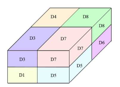
Fig. 6. Demonstration of extracting subhypercuboid
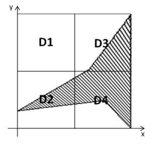
Fig. 7. A demonstration of the consistency checking algorithm problem
At this stage, initially, the portion of each consistent hyper cuboid is computed in the test data generation, then the test data is generated at randomly and equal to the calculated number of these hyper cuboids. It is possible that the generated test data from a hyper cuboid can not be able to satisfy the relevant path constraints, which in this case, will be deleted as a rejected test data. This case happens in consistent hyper cuboids that are not completely within the allowable area. After generating test data for the selected path, if the path selection operations is done equal to the number of Cyclomatic complexity, the algorithm terminates. Otherwise, algorithm goes to the path selection stage and selects the next path.
The proposed approach has been implemented by the DPRT algorithm this is shown in Algorithm 1.
DPRT(V[VarCnt], CHCs[CHC][2][VarCnt], PC[m], N, K){ Label up all error-prone nodes and edges.
for (int i = 0; i < k; i++){
HCs[CHC * pow(2, VarCnt)][2][VarCnt] =
Cartesian(V[VarCnt], CHCs[CHC][2][VarCnt]);
CHCs[CHC][2][VarCnt] = Cansistent(HCs[CHC * pow(2,
VarCnt)][2][VarCnt], PC[m]);
} /*End of while*/
PN = The portion of each hypercuboid in test data generation.
while (PN > 0){
Pick up uniformaly t at random from CHC[i][2][VarCnt];
if (PC is satisfied by t){ add t to T;
PN = PN – 1;
} /*End of if*/
} /*End of while*/ return T;
}
Algorithm 1. The DPRT proposed algorithm
This algorithm has been implemented with divide-and-conquer technique. DPRT algorithm takes the following parameters as input:
-
• V[VarCnt] : Is a one-dimensional dynamic array with length VarCnt that keeps the names of variables in path's conditions. Variable VarCnt also contains the variables count of these conditions.
-
• CHCs[CHC][2][VarCnt] : Is a 3-dimensional
dynamic array that keeps the consistent hypercuboids. Variable CHC is equal to the number of consistent hypercuboids at any time. This variable is defined as global. Since the first obtained hypercuboid from the constraint propagation process is certainly consistent, the initial value of CHC is considered equal to one. For storage a hypercuboid, it is enough that the minimum and maximum values of all the involved variables to be stored in it. Therefore the second dimension of this array is considered equal to 2 (one for minimum value and another for maximum value). Since the number of hypercuboids variables of a path is always constant the second and third dimensions of this array are considered as constant. Also, because the number of consistent hypercuboids are continuously changing, the first dimension of this array is dynamically defined.
-
• PC[m] : The dynamic array contains conditions of the relevant path that is obtained from the symbolic execution process.
-
• N : This variable keeps the number of requested test data. DPRT algorithm will eventually generate N test data.
The other parameters are also used locally in this algorithm that the most important of them are as follows:
-
• HCS[CHC * pow(2,VarCnt)][2][VarCnt] : Is a 3dimensional dynamic array that keeps the generated hyper cuboids obtained from the Cartesian product of the consistent hyper cuboids subdomains within. As mentioned, the number of obtained hyper cuboids from the CHC consistent hyper cuboids will be equal to CHC × 2VarCnt. Therefore the first
dimension of this array is changed dynamically and at this amount every time. The second and third dimensions of this array are defined like the CHC array.
-
• PN : This variable at any time, first keeps the portion of selected hyper cuboid in test data generation. After generating each test data, the PN is decreased one.
It should be noted that the mentioned parameters and variables, have been also used with the same name in the next annotated functions.
The method of DPRT algorithm is in this way that first, it performs the labeling operation of error-prone nodes based on the mentioned explanations. At the following, with help of two functions Cartesian and Consistent, the consistent hyper cuboids are extracted. Extracting the consistent hyper cuboids by these two functions is repeated k times. The process initially is so that by the Cartesian function all of the consistent hyper cuboids in the CHCs array are divided to the subhypercuboids and the result is stored in the array HCs. Then, with using of the consistency checking function “Consistent”, the consistent hyper cuboids of HCs array is extracted and again is stored in the CHCs array. The algorithms and the detailed operations of these functions will be described later. After extracting the consistent hyper cuboids, the portion of each one is calculated in test data generation and is stored in the variable PN. Finally after selecting the first hyper cuboid, test data will be generated by random function in Turbo C + + and randomly from it. If the generated test data, be able to satisfy all the conditions in array PC[m], it has been accepted as an acceptable test data and one value is decreased from value PN. When PN = 0, means that the test data is generated to the desired number from the selected hyper cuboid. In this case, the next hyper cuboid is selected and test data generation process from it will be resumed. This process is repeated until the selection of the last hyper cuboid and its test data generation (i.e. CHC times). The set of generated test data is returned by the variable T.
As mentioned, DPRT algorithm uses two Cartesian and Consistent functions for extracting consistent hypercuboids. In the following we describe the operation of these functions. You can see the Cartesian function algorithm in Algorithm 2.
Cartesian(V[VarCnt], CHCs[CHC][2][VarCnt]){
Momory Allocation for HCs;
for (i = 0; i < CHC; i++)
for (k = 0; k < VarCnt; k++)
for (j = 0; j < pow(2, VarCnt); j++){
ZorO = (j / pow(2, VarCnt - k - 1) % 2;
HCs[j + (i * pow(2, VarCnt))][0][k] = a[i][0][k] + ZorO * ceil((a[i][1][k] – a[i][0][k]) / 2);
HCs[j + (i * pow(2, VarCnt))][1][k] = a[i][0][k] - (1-ZorO) * (floor((a[i][1][k] – a[i][0][k]) / 2)+1);
} /*End of for j*/ return HCs;
}
Algorithm 2. The Cartesian function
In this algorithm first, the memory is allocated to the array HCs. CHC × 2VarCnt elements are allocated to the first dimension of the array that is equal to the number of the hyper cuboids which is supposed to be generated. The number of next loops iterations has also been set by this value. If the minimum and maximum domain of each variable be divided into two subdomains, a hyper cuboid is obtained from the Cartesian product in one of the two subdomains of all variables. Namely from the first variable, one of the first or second subdomain, from the second variable also one of its subdomains, and similarly from the variable VarCnt also one of its subdomains are selected. Selected set gives a new hyper cuboid. This issue that which subdomain of a variable should be selected at any time is determined by variable ZorO. If the value of this variable be equal to zero, the result of 1-ZorO will be equal to one. In this case the first subdomain will be selected. Also, if the variable ZorO value be equal to one, the 1-ZorO result will be equal to zero, in which case the second subdomain will be selected. Finally, the generated hyper cuboids are returned as output by the array HCs. You can see the second used function algorithm namely the Consistent function in Algorithm 3.
Consistent algorithm initially allocates memory to the CHCs array. The count of first dimension of array elements will also be considered equal to HCs array; because it is possible that all hyper cuboids of array HCs be consistent. Because in this function, the extracting process of consistent hyper cuboids will be resumed, variable CHC is initialized with 0. Also the number of consistent and external hyper cuboids will be equal to 2VarCnt. It should be mentioned that the variable EHC at any time is equal to the number of external hyper cuboids. This variable is not essential and only is used to control the algorithm operation correctness. Because the total sum of variables CHC and EHC always will be an exponential of two. The algorithm process continuation is designed in this way that if the corner of a hyper cuboids cannot able to satisfy all of the path conditions, the variable external will be incremented. Otherwise, the variable internal will be decremented. It is clear that if variable external == 2VarCnt it means that all points of selected hypercuboid are external. In this case the variable EHC will be incremented. Otherwise the hypercuboid will be stored as a consistent hypercuboid in the array CHCs. Similarly in this case the variable CHC will be incremented. After extracting all the consistent hypercuboids and store those in array CHCs, this array will be returned as output.
Consistent(HCs[CHC * pow(2, VarCnt)][2][VarCnt], PC[m]){ Momory Allocation for CHCs;
CHC = 0;
for (i = 0; i < brows; i++){ for (r = 0; r < pow(2, VarCnt); r++){ expr1 = (PC[0] if (! expr1)
external++;
else internal++;
} /*End of for r*/ if (external == pow(2, VarCnt))
EHC++;
else{ for (j = 0; j < cols; j++)
for (k = 0; k < pow(2, VarCnt); k++){ CHCs[CHC][j][k] = HCs[i][j][k]; CHC++;
} /*End of for k*/
} /*End of if*/
} /*End of for i*/ return CHCs;
}
Algorithm 3. The Consistent function
-
IV. Results
-
4.1. Evaluation Criteria
In this section, we measure the performance of proposed approach based on two criteria. To do this, we perform experiments on four programs. The first program being tested is Foo function which contains a mutant error. The second program is Triangle which has been proposed by Myers [2]. This program contains arithmetic overflow errors. The next program being tested is an aircraft collision avoidance system called Tcas. This program has been selected from the Siemens test suite [32]. The Siemens programs were assembled by Tom Ostrand and some coworker’s at Siemens Corporate Research for the purpose of studying the fault detection capabilities of control-flow and data-flow coverage criteria. Tcas is made up of 173 lines of C code and has a 41 error version which can be downloaded from Software-artifact Infrastructure Repository [33]. Different versions of Tcas contain variable errors that have been seeded there by expertise. The last program also being tested is Totinfo which has been selected from the Siemens test suite. Totinfo reads a large number of numeric data tables as input and computes the given statistical input data. It also computes statistics for each table as well as across all tables. This program is made up of 406 lines of C code and has a 23 error version which also can be downloaded from Software-artifact Infrastructure Repository. Finally, an experiment will perform on abilities of DPRT than other approaches to discover the faulty versions.
To evaluate the proposed approach more precisely, the experiments have been done on both the Random Testing (RT) and Path-oriented Random Testing (PRT) [21] methods as well as the DPRT method. Random Testing (RT) attempts to generate test data at random according to a uniform probability distribution over the input variables domain. The PRT method aims at uniformly generating of random test data that execute a single path within a program. The main goal of PRT is minimize the amount of rejected test data. In order to get better results, the parameter k in the DPRT and PRT methods for function Foo is considered the value 6. This parameter for the Triangle, Tcas and Totinfo is 5, 2 and 3 values, respectively.
To be fair, the same situations have been applied for the implementation of all these methods. All of these algorithms will be implemented by Turbo C++ 4.5 language on a Pentium IV personal computer with 1.6 GHz CPU and 288 MB RAM (a 256 MB RAM with a 32 MB RAM). Also the random function in this programming language is used for random generation. All programs take variables name, their ranges, the path conditions, the number of requested test data and splitting parameter k as input and generate test data to the requested number. It should be noted that the best division parameter value will be considered for PRT.
In many previous methods [34, 35], the sum of the rejected test data has been considered as one of the evaluation criteria. Though, it is a good criterion, it is not enough. For example, if the number of rejected test data, be equal to zero in an ideal limit but the generation test data, not be lead to the discovery of error, a wasted work is almost done. As mentioned before, software testing that doesn’t lead to error detection can’t be a suitable test. However, this criterion has been introduced because it is effective especially in the running time of the algorithm. In other words, whatever the number of rejected test data be larger, more time also will be spent for generating test data at the requested amount. Therefore, we present an error detection rate (EDR) criterion based on the following equation:
the number of diagnostic test data
EDR = --------------------------------- the number of the total generated test data
This criterion defines the error detection probability of a test data. In this criterion, the number of rejected test data has also been considered automatically. Because the total number of rejected test data and the number of acceptable test data, give the total number of generated test data; and since this parameter is in the denominator, its increase is caused to reduce diagnostic rate and its reduction is caused to increase this rate. Thus, according to this criterion, try to reduce the number of rejected test data. On the other hand, the number of diagnostic test data has a direct relationship with error detection rate. So should be tried to increase the number of diagnostic test data. The next criterion, called error detection speed (EDS), is defined according to the following equation:
the number of diagnostic test data
EDS = --------------------------- running time
The number of rejected test data and consistency checking algorithm run time are two effective run time factors. It is clear that if the number of using the consistency checking algorithm increases, assuming the constant number of rejected test data, algorithm running time will also be increased. Whereas measuring the run time of the consistency checking algorithm needs a real execution and is not assessable by mathematical equations, we will measure this parameter with a real execution in this section. Memory usage criterion is also considered a criterion which is not very important that due to its low importance we are not considering it in this field.
The abbreviation N represents the total number of the acceptable test data generation, E shows the number of diagnostic test data, T represents running time that measured in second, R represents the number of rejected test data, EDR represents the error detection rate and EDS shows the error detection speed. Remember that the values of these variables is equal to EDR = E/(N+R) and EDS = E/T .
-
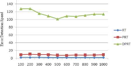
4.2. Experiments Results on Function Foo
-
4.3. Experiments Results on Program Triangle
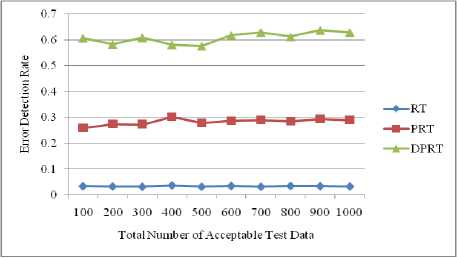
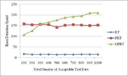
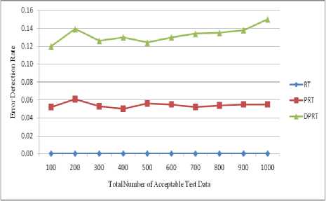
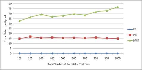
Arithmetic overflow error is another common error in programming (row 1 of Table 1). The Triangle program that was written by Myers contains these kinds of errors. This program checks the possibility of constructing a triangle by three received input numbers. Consider the experiment results of the related methods on this program in Table 3. These results have been collected by running the algorithm for N=100 to N= 1000 with a step interval of 100.
One of the common mistakes of programming is lack of using the symbol "{}" in conditional and iteration loops structures containing more than one instruction
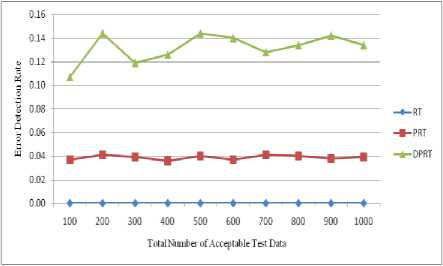
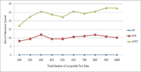
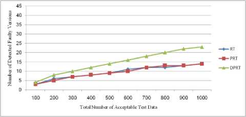
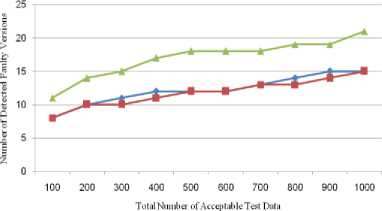
(row 3 of Table 1). The shown Foo function shows this mistake in the Fig. 1. In this function, sequential instructions x-- and cout< Fig. 8 and Fig. 9 show the error detection rate of the aforementioned methods and their error detection speed based on the total number of acceptable test data, respectively. Observing the results of these experimental methods on function Foo, the conclusion can be made that the error detection rate of the DPRT method is about 97 times more than the RT method and about 21 times more than the PRT method. It is also observed that the error detection speed of the DPRT method is about 66 times more than the RT method and 13 times more than the PRT method. The error detection rate of the before mentioned methods and their error detection speed based on the total number of acceptable test data is illustrated in Fig. 10 and Fig. 11, respectively. Table 2. Experiments results of function Foo N 100 200 300 400 500 600 700 800 900 1000 RT E 3 7 11 12 13 17 20 24 26 31 R 664 1449 2124 2809 3617 4321 4977 5814 6319 7114 Ts 1.47 3.61 5.19 7.1 9.39 11.01 12.79 14.21 16.46 17.81 EDR 0.004 0.004 0.005 0.004 0.003 0.003 0.004 0.004 0.004 0.004 EDS 2.04 1.94 2.12 1.69 1.38 1.54 1.56 1.69 1.58 1.74 PRT E 3 8 10 13 14 16 21 23 27 32 R 69 153 239 294 373 497 527 632 687 755 Ts 0.33 0.77 1.07 1.43 1.87 2.19 2.59 2.91 3.3 3.62 EDR 0.018 0.023 0.019 0.019 0.016 0.015 0.017 0.016 0.017 0.018 EDS 9.09 10.39 9.35 9.09 7.49 7.31 8.11 7.9 8.18 8.84 DPRT E 65 138 195 242 291 366 417 482 571 636 R 54 146 180 263 329 408 493 553 575 654 Ts 0.51 1.08 1.69 2.22 2.88 3.37 3.87 4.36 5.02 5.59 EDR 0.422 0.399 0.406 0.365 0.351 0.363 0.35 0.356 0.387 0.385 EDS 127.45 127.78 115.38 109.01 101.04 108.61 107.75 110.55 113.75 113.77 Table 3. Experiments results of program Triangle N 100 200 300 400 500 600 700 800 900 1000 RT E 53 107 162 233 261 336 382 46 503 537 R 1511 3131 4915 6133 7837 9361 11719 12734 14247 15871 Ts 3.12 7.35 10.91 15.34 18.82 23.31 26.67 30.14 33.25 36.7 EDR 0.033 0.032 0.031 0.036 0.031 0.034 0.031 0.034 0.033 0.032 EDS 16.99 14.56 14.85 15.19 13.87 14.41 14.32 15.3 15.13 14.63 PRT E 52 109 164 229 271 340 389 445 494 559 R 101 197 300 355 472 583 641 758 778 930 Ts 0.33 0.71 1.05 1.48 1.92 2.25 2.52 2.92 3.3 3.68 EDR 0.259 0.275 0.273 0.303 0.279 0.287 0.29 0.286 0.294 0.29 EDS 157.58 153.52 156.19 154.73 141.15 151.11 154.37 152.4 149.7 151.9 DPRT E 88 162 251 327 415 515 601 675 789 873 R 45 78 113 163 221 235 256 303 339 387 Ts 0.82 1.29 1.59 1.98 2.36 2.75 3.13 3.46 3.78 4.17 EDR 0.607 0.583 0.608 0.581 0.576 0.617 0.629 0.612 0.637 0.629 EDS 107.32 125.58 157.86 165.15 175.85 187.27 192.01 195.09 208.73 209.35 Fig. 8. Error detection rate chart of function Foo Total Number of Acceptable Test Data Fig. 9. Error detection speed chart of function Foo Fig. 10. Error detection rate chart of program Triangle Fig. 11. Error detection speed chart of program Triangle With the experiments results of these methods about the program Triangle, a conclusion can be made that error detection rate of the DPRT method is about 19 times more than the RT method and about 2 times more than the PRT method. It is also observed that error detection speed of the DPRT method is about 12 times more than the RT method and 1.1 times more than the PRT method. Moreover, error detection speed of the DPRT method increases more with a greater amount of test data rather than the other two methods. 4.4. Experiments Results on Program Tcas Tcas program is constructed of 9 functions and 14 global integer variables. The alt-sep-test function has been selected to perform the testing. This function will call 4 more after getting called, from which 2 functions of those 4 call functions will call another 6 functions. You consider the experimental results on this function in Table 4. Due to time consuming experiments regarding this function, the results have been recorded for N=100 to N=1000 with a step interval of 100. 4.4. Experiments Results on Program Totinfo Fig. 12 and Fig. 13 show the error detection rate of the aforementioned methods and their error detection speed based on the total number of acceptable test data, respectively. With the experiments results of these methods about the program Tcas, a conclusion can be made that the error detection rate of the DPRT method is about 7400 times more than the RT method and about 3.4 times more than the PRT method. It is also observed that error detection speed of the DPRT method is about 417 times more than the RT method and 2.4 times more than the PRT method. Moreover, error detection speed of the DPRT method increases more with a greater amount of test data rather than the other two methods. The Totinfo program has been constructed of 7 functions, 2 arrays and 2 global variables. The InfoTbl function has been selected to perform the testing. This function contains nested loops and also conditional statements. You consider the experimental results on this function in Table 5. Due to time consuming experiments regarding this function, the results have been recorded for N=100 to N=1000 with a step interval of 100. The error detection rate of the aforementioned methods with the total number of acceptable test data has been shown in the Fig. 14. In This experiment, the error detection speed of the total number of acceptable test data has been shown in the Fig. 15. Table 4. Experiments results of program Tcas N 100 200 300 400 500 600 700 800 900 1000 RT E 33 62 91 117 162 184 219 247 281 316 R 1721637 3470225 5399979 6737013 8731610 10473727 11587160 13562658 15297654 17101046 Ts 591.4 1205.7 1574.0 2470.9 2858.8 3486.3 3642.5 4015.6 4266.9 5080.6 EDR 0.000 0.000 0.000 0.000 0.000 0.000 0.000 0.000 0.000 0.000 EDS 0.06 0.05 0.06 0.05 0.06 0.05 0.06 0.06 0.07 0.06 PRT E 31 65 93 121 157 185 223 256 273 318 R 734 1385 2091 2919 3417 4458 4711 5539 6230 7164 Ts 3.8 6.9 7.8 12.9 16.7 17.5 20.2 21.6 25.3 31.2 EDR 0.037 0.041 0.039 0.036 0.04 0.037 0.041 0.04 0.038 0.039 EDS 8.16 9.42 11.92 9.38 9.4 10.57 11.04 11.85 10.79 10.19 DPRT E 81 175 235 319 407 531 582 671 793 864 R 654 1012 1671 2125 2317 3192 3850 4191 4704 5428 Ts 4.7 7.8 9.2 13.4 18.3 20.7 24.0 26.3 28.7 31.5 EDR 0.107 0.144 0.119 0.126 0.144 0.14 0.128 0.134 0.142 0.134 EDS 17.23 22.44 25.54 23.81 22.24 25.65 24.25 25.51 27.63 27.43 Table 5. Experiments results of program Totinfo N 100 200 300 400 500 600 700 800 900 1000 RT E 25 55 74 98 125 157 183 199 230 242 R 756560 1558513 2118368 3250584 3809768 4577188 5273223 6060045 6740949 7452172 Ts 265.2 542.6 782.6 1113.4 1307.9 1629.5 1840.2 2135.2 2347.1 2585.9 EDR 0.000 0.000 0.000 0.000 0.000 0.000 0.000 0.000 0.000 0.000 EDS 0.09 0.10 0.09 0.09 0.10 0.10 0.10 0.09 0.10 0.09 PRT E 24 56 77 98 127 149 176 202 222 247 R 360 711 1152 1548 1767 2124 2664 2916 3168 3509 Ts 1.6 3.3 4.9 6.1 8.1 9.4 11.3 12.6 14.5 16.5 EDR 0.052 0.061 0.053 0.050 0.056 0.055 0.052 0.054 0.055 0.055 EDS 15.00 16.97 15.71 16.07 15.68 15.85 15.58 16.03 15.31 14.97 DPRT E 59 128 173 229 270 326 385 473 534 652 R 393 724 1073 1359 1670 1909 2172 2712 2956 3342 Ts 1.8 3.5 4.4 6.2 7.1 8.2 10.0 11.3 12.4 13.9 EDR 0.120 0.139 0.126 0.130 0.124 0.130 0.134 0.135 0.138 0.150 EDS 32.78 36.57 39.32 36.94 38.03 39.76 38.50 41.86 43.06 46.91 Fig. 12. Error detection rate chart of program Tcas With the experiments results of these methods about the program Totinfo, a conclusion can be made that the error detection rate of the DPRT method is about 3700 times more than the RT method and about 2.4 times more than the PRT method. It is also observed that error detection speed of the DPRT method is about 415 times more than the RT method and 2.5 times more than the PRT method. Moreover, error detection speed of the DPRT method increases more with a greater amount of test data rather than the other two methods. Nonetheless, outcomes from experiments on larger benchmarks need to be verified. Fig. 13. Error detection speed chart of program Tcas Fig. 14. Error detection rate chart of program Totinfo experiments in this direction could be to give more accurate results. V. Threats to Validity 4.6. Experiments on the Rate of Faulty Versions Detection The programs Tcas and Totinfo contain 41 and 23 faulty versions, respectively. Only one seeded error exist in majority of these versions. The ability of different approaches to discover the faulty versions is one criterion for the comparison. Fig. 16 and Fig. 17 show the number of Tcas and Totinfo faulty versions that are detected against the different numbers of test cases generated using the RT, PRT and DPRT methods. These results have been collected by running the algorithms for N=100 to N= 1000 with the step interval of 100. In our studies this section is dedicated to threat to validity, including external and internal validity. We use Turbo C++ 4.5 to implement our tools for test data generation. Threats to internal validity concern with possible errors in our implementations that could affect our finding. Nevertheless, we carefully checked most of our outcomes for decreasing these threats considerably. The result show the number of faulty versions detected by DPRT method is higher than the PRT and RT methods. Furthermore, the detection rate has higher grown at the first and this rate is decreased when the number of generated test cases is increased in these experiments. In the experiments on Totinfo, this observation is more heighted. Therefore, it can be concluded the number of versions that have been discovered in the early of generating test cases is higher than the last ones. Further Fig. 15. Error detection speed chart of program Totinfo Fig. 16. Number of faults detected in the program Tcas Fig. 17. Number of faults detected in the program Totinfo Our experiments are restricted to only five small or medium-sized programs which is the main threat to external validity. More experiments on larger programs may further strengthen the external validity of our findings. Further investigations of other programs in different programming languages would help generalize our results. Moreover, these programs were originally written in C, object-oriented features such as inheritance, polymorphism and associations did not used. Therefore, the results may not generalize our finding. Additionally, there is exactly one seeded fault in every Siemens program; in practice, programs contain much more complex error patterns. VI. Conclusions And Future Works In this paper, a new approach has been proposed for path-oriented test data generation. The main goal of the proposed approach was generating test data that lead to error detection in the least amount of time. In different programming languages, some of the instructions are more error-prone. Therefore, to generate test data, as much as possible the paths that contain these instructions were selected. After generating hyper cuboids from the allowable area, the relevant test data were generated by them. After explaining the proposed algorithm, it was evaluated and compared to other related works based on new and important criteria. To evaluate the interest rate of different methods to the error detection, two criteria, error detection rate and error detection speed are defined. In the following, to evaluate the mentioned criteria more exactly, some experiments were done on both the four functions. On average, according to these experiments, error detection rate of the DPRT method obtained is about 2804 times more than the RT method and about 7.2 times more than the PRT method. The error detection speed of this method is obtained about 228 times more than the RT method, on average, and 4.8 times more than the PRT method. Therefore according to the values obtained of the completed experiments, the important goals such as discovering more errors in less time, decreasing test costs, reducing wasted resources, increasing the error detection speed and on time or even in time delivery of the product to the customer was a success. For future works, extending the proposed approach so that having the support capability of the error-prone instructions of all programming languages will be proposed. Presenting a solution to solve the undesirable elimination of some hyper cuboids by the proposed consistency checking algorithm also will help the quality of the test process.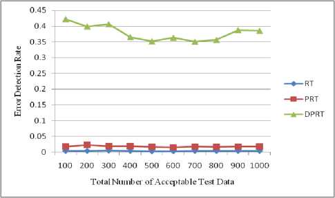
References Diagnostic Path-Oriented Test Data Generation by Hyper Cuboids
- J. Zhang and X Wang, "A Constraint Solver and its Application to Path Feasibility Analysis," International Journal of Software Engineering Knowledge Engineering, 2001 Apr; 11 (2): 139-56.
- G. J. Myers, The Art of Software Testing, 2rd ed., New Jersey: John Wiley and Sons; 2004.
- J. Peleska, E. Vorobev, and F. Lapschies, "Automated Test Case Generation with SMT-Solving and Abstract Interpretation," In: Bobaru M, Havelund K, Holzmann GJ, Joshi R, editors. Nasa Formal Methods. Third International Symposium: NFM; 2011 Apr; Pasadena, CA. USA: Springer; 2011. p. 298-312.
- N. K. Gupta and M.K. Rohil, "Using Genetic Algorithm for Unit Testing of Object Oriented Software," In: Proceedings of the 1st International Conference on Emerging Trends in Engineering and Technology (ICETET '08); 2008 Jul 16-18; Nagpur, Maharashtra. India: IEEE; 2008. p. 308-13.
- M. Prasanna and K.R. Chandran, "Automatic Test Case Generation for UML Object diagrams using Genetic Algorithm," Int J Advance Soft Comput Appl. 2009 Jul; 1 (1): 19-32.
- M. C. F. P. Emer and S.R. Vergilio, "Selection and Evaluation of Test Data Based on Genetic Programming," Software Quality Journal. 2003 Jun; 11 (2): 167-86.
- J. H. Andrews, C. H. Li. Felix, and T. Menzies, "Nighthawk: a two-level genetic-random unit test data generator," In: Stirewalt REK, Egyed A, Fischer B, editors. 22th IEEE/ACM International Conference on Automated Software Engineering (ASE); 2007 Nov 5-9; Atlanta, Georgia. USA: ACM; 2007. p. 144-53.
- C. Csallner and Y. Smaragdakis, "JCrasher: an automatic robustness tester for Java," Software Practice and Experience. 2004 Sep; 34 (11): 1025–50.
- T. Y. Chen, F. C. Kuo, and H. Liu, "Distributing test cases more evenly in adaptive random testing," Journal of Systems and Software. 2008 Dec; 81 (12): 2146-62.
- H. I. Bulbul and T. Bakir, "XML-Based Automatic Test Data Generation," Computing and Informatics. 2008 Jan; 27 (4): 660-80.
- P. Nirpal and K. Kale, "Comparison of Software Test Data for Automatic Path Coverage Using Genetic Algorithm," International Journal of Computer Science and Engineering Technology. 2011 Feb; 2 (2): 42-8.
- J. Edvardsson, "A Survey on Automatic Test Data Generation," In: Proceedings of the Second Conference on Computer Science and Engineering in Linkoping; 1999. p. 21-28.
- N. T. Sy and Y. Deville, "Consistency Techniques for interprocedural Test Data Generation," Proceedings of the Joint 9th European Software Engineering Conference and 11th ACM SIGSOFT Symposium on the Foundation of Software Engineering (ESEC/FSE03); 2003 Sep 1-5; Helsinki, Finland. Finland: ACM; 2003.
- P. Hentenryck, V. Saraswat , and Y. Deville, "Design, implementation, and evaluation of the constraint language cc(fd)," Journal of Logic Programming. 1998 Oct 1; 37 (1-3): 139–64.
- F. Zareie and S. Parsa, "A Non-Parametric Statistical Debugging Technique with the Aid of Program Slicing (NPSS)", IJIEEB, vol.5, no.2, pp.8-14, 2013. DOI: 10.5815/ijieeb.2013.02.02.
- I. Alsmadi and S. Alda, "Test Cases Reduction and Selection Optimization in Testing Web Services", IJIEEB, vol.4, no.5, pp.1-8, 2012.
- S. Tanwer and D. Kumar, "Automatic Test Case Generation of C Program Using CFG," International Journal of Computer Science. 2010 Jul; 7 (8): 27-31.
- R. Blanco, J. Tuya, and B. A. Diaz, "Automated Test Data Generation Using a Scatter Search Approach," Information and Software Technology. 2009 April; 51 (4): 708-20.
- D. Gong, W. Zhang, and X. Yao, "Evolutionary generation of test data for many paths coverage based on grouping," Journal of Systems and Software. 2011 Dec; 84 (12): 2222-33.
- L. Cai, "A Business Process Testing Sequence Generation Approach Based on Test Cases Composition," First ACIS/JNU International Conference on Computers, Networks, Systems and Industrial Engineering (CNSI); 2011 May 23-25; Jeju, Island. Korea: IEEE; 2011. p. 178-85.
- A. Gotlieb and M. Petit, "A Uniform Random Test Data Generator for Path Testing," Journal of Systems and Software. 2010 Dec; 83 (12): 2618-26.
- R. Zhao and Y. Huang, "A Path-oriented automatic random testing based on double constraint propagation," International Journal of Software Engineering & Applications. 2012 Mar; 3 (2): 1-11.
- M. Alzabidi, A. Kumar, and A. D. Shaligram, "Automatic Software Structural Testing by Using Evolutionary Algorithms for Test Data Generations," International Journal of Computer Science and Network Security. 2009 Apr; 9 (4): 390-5.
- J. N. Swathi, T. I. Sumaiya, and S. Sangeetha, "Minimal Test Case Generation for Effective Program Test using Control Structure Methods and Test Effectiveness Ratio," International Journal of Computer Applications. 2011 Mar; 17 (3): 48-53.
- M. Catelani, L. Ciani, V. L. Scarano, and A. Bacioccola, "Software automated testing: A solution to maximize the test plan coverage and to increase software reliability and quality in use," Computer Standards & Interfaces. 2011 Feb; 33 (2): 152-8.
- P. N. Boghdady, N. L. Badr, M. Hashem, and M. F. Tolba, "A Proposed Test Case Generation Technique Based on Activity Diagrams," International Journal of Engineering & Technology. 2011 Jun 10; 11 (3): 37-57.
- M. Ehmer-Khan, "Different Approaches to White Box Testing Technique for Finding Errors," International Journal of Software Engineering and Its Applications. 2011 Jul; 5 (3): 1-14.
- N. Mansour and M. Salame, "Data generation for path testing," Journal of Software Quality. 2004 Jun 1; 12 (2): 121-36.
- S. Oualline, How Not to Program in C++, ISBN 10:1886411956. U.S.: No Starch Press; 2003.
- H. Zhu, P. A. V. Hall, and J. H. R. May, "Software Unit Test Coverage and Adequacy," ACM Computing Surveys. 1997 Dec; 29 (4): 366-427.
- F. Elberzhager, S. Kremer, and J. Munch, and D. Assmann, "Focusing Testing by Using Inspection and Product Metrics," International Journal of Software Engineering and Knowledge Engineering. 2013; 23 (04): 433-462.
- M. Hutchins, H. Foster, T. Goradia, and T. Ostrand, "Experiments on the effectiveness of dataflow- and control flow-based test adequacy criteria," In: Proceedings of the 16th International Conference on Software Engineering; 1994. p. 191-200.
- M. B. Dwyer, S. Elbaum, J. Hatcliff, G. Rothermel, H. Do, and A. Kinneer, "Software-artifact infrastructure repository," Available at http://sir.unl.edu/portal/index.php, Last visited:Dec 2012.
- M. N. Ngo and H. B. K. Tan, "Heuristics-based infeasible path detection for dynamic test data generation," Original Research Article Information and Software Technology. 2008 Jun 25; 50 (7-8): 641-55.
- R. S. Landu, "Analysis of Rejected Defects in First and Second Half Builds of Software Testing Phase," Journal of Computing Technologies. 2012 Aug 31; 1 (4): 45-51.
