Digital Control and Management of Water Supply Infrastructure Using Embedded Systems and Machine Learning

Published Online on October 8, 2023 by MECS Press

Water is an essential resource and everyone has access to clean and pollution-free water through the use of pipe distribution networks. These pipework’s are buried underground for several years and thus, due to aging, corrosion issues, and third-party damage, cracks occur along the pipes, which causes the loss of significant volumes of water.

Since they are underground and are not readily accessible, monitoring becomes a serious challenge. In a severe situation, the problem becomes more complex when leaks occur significantly at several points along the pipes resulting in supply shortages and contamination as alluded by authors in [1-4]. In view of this, this research targets to provide a solution by focusing on mechanisms to detect and shut fluid leakage when they occur due to breakage of pipeline using hydrostatic pressure and digital control system methods. Existing industrial scale infrastructure for water, oil and gas supply pipeline implementations researched are mostly reliant on destination endpoint supervision systems as means of detecting comprise in the flow of supply received from the production end. This is common with waterboard, oil and gas companies especially in developing countries like Nigeria. The methodology proposed in this research brings an improvement over the legacy method by facilitating real-time and direct detection and shutdown of flow through any physically compromised or broken pipeline which may be situated in remote location far away from user or destination endpoint of the infrastructure and restores flow automatically when fault point is resolved. Fault incidents are recorded in a progressive database to enable pattern modelling using Machine learning for efficient maintenance planning and infrastructure management. While this proposed method proves potent in its functionality, it does not identify the exact point of breakage along the pipeline segments. Fault point identification is an area being considered in future research, as an evolution of the methodology proposed in the current research work.

This paper is structured into five sections beginning with Section 1 covering introduction, Section 2 covers the theoretical background of the research. The method used in actualizing the background principles is covered in Section 3. Experimentation results discussions and conclusion are covered in sections 4 and 5 respectively.

2.    Theoretical Background

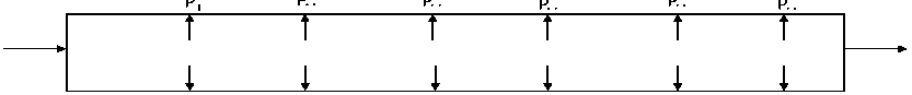
The theoretical framework of this research is centred on fault detection and control, as the core objective of this work is solving the problem of water supply infrastructure efficiency orchestrated by distribution losses along pipelines. Leveraging Pascal principles and the concepts of hydraulics elaborated by Serrin.[5], a pipeline segment can be analytically represented by indications of various hydrostatic pressure components exerted around the pipe segment by water passing through it as shown in fig.1.

P in

р out

P..              P..

P..                ^P..                   P..

P n

Fig.1. Pressure components in a field pipe segment

Based on Pascal's theorem of hydrostatic equilibrium, at a steady state, the sum of hydrostatic pressure components equates to zero as shown in equation (1).

P in + P 1 +P 2 + P 3 + …. P n + P out = 0                                        (1)

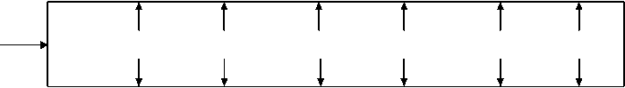
Meaning that, ∑ P i = 0. At a steady state, the liquid water flowing through the pipe exerts undiminished hydrostatic pressure along the interior wall of the pipe while it flows through it. This state is maintained irrespective of the geometric shape taken by the pipe, but this equilibrium state is disrupted once the pipe segment is breached by way of break or rupture. From the prototype schematics shown in fig.3, the pressure components on the pipe section illustrated in fig.4 can be analyzed using the Pascal principle stated in equations (1) to (7). In the analysis below, atmospheric pressure on the water surface in Tanks A and B as shown in fig.2 is represented by P A and P B in fig.4. This establishes a hydrostatic equilibrium condition equivalent to the pressure equilibrium established by a steady flow of water through an unperturbed pipe. P S and P L are values of pressure at the sensor and leak points respectively.

P A and P B represent the sum of atmospheric pressure and pressure due to the column of water in containers A and B respectively. Based on Pascal’s principle, the pressure values at these points of focus are represented in equations (2) and (3)

P A - P S - P L + P B = 0                                              (2)

P A + P B = P S + P L                                              (3)

When the Leak Valve LV is in a closed position, P L = 0 as there is no leak. The sensor pressure value is P S1 at this time, and when in an open position P L is not zero, and the sensor pressure is P S2 . The value of P S1 is greater than P S2 . The differential pressure ∆P S is the parameter used by a software program in the Embedded systems microcontroller to open or close the control value based on the control algorithm. This is mathematically explained by equations (4) to (7).

P S = P A + P B - P L                                              (4)

P S1 = P A + P B

As P L is Zero due to no leak, P S1 changes to a new value P S2 when is open, P L is no longer zero.

P S2 = P A + P B - P L

Legend

∆P S = P S1 - P S2 = (P A + P B ) - (P A + P B - P L )

Tank A

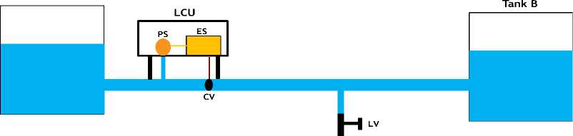
LCU – Line Control Unit

PS – Pressure Sensor

ES – Embedded System

CV – Control Valve

LV – Leak Valve

Fig.2. Schematics of prototype pipeline segment

P S                ^P..                  P..                P..                  P..               P..

P A

◄ ---- PB

P..               P..

P..               ^P..                 P..             P L

• Fig.3.    Pressure components in a prototype pipe segment

P A 1 I PS            I PB

P L

• Fig.4.    Pressure components analysis of a prototype pipe segment

In Mathematical terms, the value of ∆P S is equal to the hydraulic pressure with which water escapes the pipe wall at the point it was opened via an experimental valve, or a rupture point due to breakage. In terms of control, the sensor threshold is set at a value equal to P S1 so that a drop from that value triggers actuation at the control valve.

Below are the Prototype design conditions considered:

• •    At steady state, P L = 0, Sensor pressure, P S1 = P A + P B

• •    At leak event state, P L ≠ 0 , Sensor pressure, P S2 = P A + P B – P L

• •    The drop in hydrostatic pressure within the pipe segment is ∆P S = P L

• •    The sensor threshold is set at P S1 and drops by P L to trigger pipe closure actuation.

• •    P A and P B are sums of Atmospheric pressure and pressure of water columns in respective tanks.

• •    P A = P B = P atm + P water , P atm = 101KPa, P water = H x d x g = 0.36 x 1000 x 10 = 3600Pa.

Where H is the height of water column in the tanks, d is the density of water and g is the acceleration due to gravity. Hence, P A = P B = P atm + P water = 101+ 3.6 = 104.6 KPa

P S1 = P A + P B = 2 x (104.6) = 209.4 KPa                               (8)

• •    Sensor maximum threshold value in the control program is set at 200KPa

• •    The capacity range of pressure sensor used in the prototype is 0 to 5MPa.

3.    Method 3.1.    Situation Analysis

Another theoretical aspect reviewed in this research was Infrastructure data which is collected and used for evaluation of the functional efficiency of the infrastructure. Data harvesting from a water supply Infrastructure just like other distributed control systems relies on the use of sensors incorporated in data acquisition devices. In a typical pipeline infrastructure using Supervisory Control and Data Acquisition (SCADA) system, Remote Terminal Unit (RTU) can be used for flow data acquisition. Harvested data are then reposited in a database platform located at the facility's central office. Such database platforms are computer systems equipped with data analysis software used for data analytics from which insights and knowledge of the infrastructure efficiency as well as its value delivery capacity are determined. Data has become a crucial commodity for decision-making at different levels of infrastructure and enterprise management as alluded by Minh Dang et al.[6] while elaborating the import of data in IoT healthcare application.

Many authors have researched water management problems in the past including the authors of [7] who designed and tested a fuzzy logic-based water pump controller to control the amount of water pumped through a point using a flow rate parameter. Patil and Bharkad [8] demonstrated the use of temperature and weight of liquid as parameters for controlling flow rate. Moon and lee [9] proposed the use of a hybrid algorithm of fuzzy and Proportional and Integral (PI) mechanisms to control the temperature of molten glass in the glass manufacturing industry. In the work of Neelshetty et al. [10], the authors researched the use of SCADA and PLC to control recycled water treatment plants. The authors of [11] based their research work on the treatment of unclean water from larger sources such as rivers, lakes, and other water bodies. A proprietary SCADA solution was used here, but this featured additional quality-testing parameters such as turbidity and chlorine content test of the treated water. The work of Shashank et al. [12] provide useful insight into the use of inexpensive hardware such as Microcontroller-based Arduino with open-source software for data acquisition. This serves as a cheaper alternative to a full-scale SCADA deployment. The work of Bakker et al. [13] demonstrated the advantage of model-based control over level-based control, as model-based control provides a more stabilized production flow as compared to level-based control. The work of Rahbalaram et al. [14] on predictive analysis for water management using Machine Learning (ML) and Survival analysis was able to show the efficacy of mining performance data related to system faults using ML algorithms. Ross et al. [15] and van de Ven et al. [16] in their work emphasized the importance of intelligent modeling techniques for determining the quality of water production in a shorter space of time with higher accuracy as compared to the use of traditional laboratory test regimes. Large data samples acquired through plant terminals were fed into an ML-driven software where pre-classified quality grades were used to determine the quality of potable water produced after a pre-determined number of treatment iterations. It provided reliable results in real-time with a high degree of accuracy.

The first focus of this work is to have a data-driven analysis of an existing pipeline infrastructure in a chosen location in a bit to study the relationship between production and distribution loss of the water supply infrastructure, and any pattern exhibited by the failure profile. The end goal is to model such patterns to enable event forecasts. Empirical data from utility supply infrastructure can be obtained from a supervisory or monitoring platform. Utility supply companies do have this provision and use different names for such platforms. The platform is used for collating and analyzing alarm data received from field RTUs. This research refers to such platform as a Central Office Monitoring Platform (COMP) and can be a software component in SCADA system which could be hosted on premise or in cloud. It provides the means for managing the field infrastructure based on information derived from harvested data. Five main attributes of data, namely: Volume, Velocity, Veracity, Variety, and Value, in the list posited by Sood et al. [17] are crucial for data reliability and analytics via the COMP. SCADA RTUs connected to a flow meter at each tail-end of the water distribution network collects consumption data which the waterboard company often used to profile and determine consumption rate and indirectly make inferences on infrastructure failure profile from changes in recorded consumption profile. While this indirect approach of fault detection may be serving its purpose, a direct detection mechanism that function within the distribution part of the infrastructure provides a more accurate and reliable data and control method for infrastructure fault management. This is where the use of LCU comes in as proposed by this research. LCUs placed at head-end of pipe segments at strategic locations will collect fault data in addition to actuation control action it performs. Field data collected using endpoint RTUs and pipeline LCUs provide better information for building a reliable predictive model for future utilization and maintenance forecasts using Machine Learning. In this research, linear regression machine learning algorithm was adopted for descriptive analysis of data, while Random Forest regression was used for predictive analysis. The performance of the prediction model achieved was evaluated using the coefficient of determination or R-square. The field data collected are shown in tables 1 and 2. Fig.7 shows a simplified Wide Area Network (WAN) architecture of the data communication Network over which field data can be backhauled to the COMP. The COMP can be accessed locally via a Local Area Network (LAN) or remotely via a secure Internet connection. For purpose of this research, raw data used for supply and fault situation analysis were obtained in CSV file format from a waterboard facility operator in southern Nigeria. The data was cleaned up and represented for analysis. Result of these analyses are available in section 4.2.

Table 1. Water supply data for a metro area facility

Year	PS	TU	Production (Litres)	DL (Litres)	Number of homes	Number of schools	Number of Hospitals	NO	NAPWS
2000	404060	3000233	3749289	749055	80812	143	18	297	81
2001	412413	3693303	4615626	922323	103103	158	20	315	88
2002	420767	3741981	4676473	934492	105192	174	21	334	92
2003	429120	3282538	4102169	819631	107280	191	27	354	98
2004	437474	3516528	4394658	878129	109369	211	31	376	104
2005	445827	4272553	5339688	1067135	111457	232	33	398	112
2006	454181	4161231	5200536	1039305	113545	256	39	422	120
2007	462534	4328865	5410078	1081213	115634	282	43	447	129
2008	470888	5622069	7022583	1400514	117722	297	44	474	139
2009	479241	5155309	6439133	1283824	119810	315	47	503	150
2010	487595	5223256	6524067	1300811	121899	338	53	533	159
2011	495948	6621455	8271816	1650361	123987	346	57	565	170
2012	504302	8151046	10183805	2032759	126076	359	62	599	182
2013	512655	8456086	10565105	2109019	128164	368	64	635	195
2014	521009	9655066	12063830	2408764	130252	375	71	673	208
2015	529362	6887782	8604725	1716943	132341	386	75	713	223
PS = Population Size			TU =	Total Utilization		NO = Number of organizations
NAPWS = No of Alternative portable water sources						DL =	Distribution Loss

Internet

Operator

RTU-1

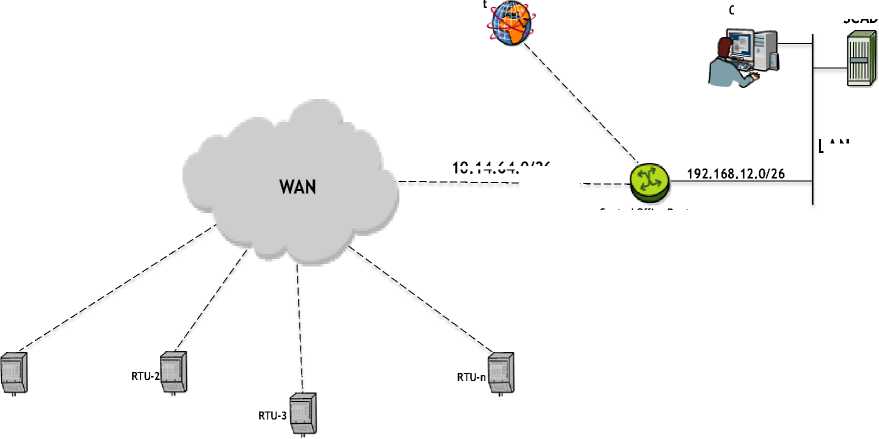
10.14.64.0/26

LAN

Central Office Router

Fig.5. Data backhaul communication network

SCADA

Fault data collected across 10 pipe cluster (PCL) areas within the 15 years period is shown in table 2 below:

Table 2. Water supply failure data for a metro area facility

Location ID	Total Segment Length (m)	Number of failures per year	Failure rate per 100m per year	Average Age of Pipe Segment (Yr.)	Average Depth from Surface (m)	MTBF (Hr)
PCL021	53777.60	8204	15.25	15	0.72	1.07
PCL022	53181.92	1620	3.06	12	0.93	5.41
PCL023	42944.48	689	1.63	13	1.10	12.71
PCL024	3768.48	128	3.38	9	0.66	68.44
PCL025	6880.16	581	8.44	7	0.98	15.08
PCL026	21604.48	954	4.44	13	0.97	9.18
PCL027	1200.00	157	2.62	11	0.56	55.73
PCL028	2450.00	321	5.35	11	1.10	27.30
PCL029	1300.00	170	2.84	12	0.00	51.45
PCL030	1058.48	139	2.31	10	0.99	63.18
Total	188165.60	12963.00	51.93

• 3.2.    Fault Detection and Resolution Mechanism

  This aspect of the research focuses on the method used to realize the LCU functionality, hence an aspect dealing with the design of fault detection and control mechanism. The LCU is achieved using a microcontroller-based embedded system. This research adopts the orifice plate method as the sensing mechanism owing to the nature of the use case in focus and the degree of accuracy required in measuring liquid flow for efficient control leveraging the work of Sood et al [17]. Actuation is based on an electro-mechanical valve sub-system. Each pipeline active junction or node comprises of an Embedded System (ES) unit, the orifice plate meter, and an electro-mechanical valve, all being incorporated together either as a retrofit or manufactured into an integrated unit referred to as the Line Control Unit (LCU) as seen in fig.6. For enterprise-grade deployments, ES units equipped with an enterprise-grade real-time operating system will be a much more suitable solution [18-20]. The Embedded System used in this work is ESP8266 equipped with an Atmel AVR microcontroller, 16 MB flash memory, and 16Mhz processor speed. The ES is then interfaced with a wireless internet modem for network communication with fault management terminals. The typical operation of the LCU stems from the operation of the algorithm programmed into the embedded system. The line control units at the head-ends of the pipeline segments are controlled locally and monitored remotely as they communicate with a back-end central office. The target is for these ES devices to communicate the status of water flow in pipe segments on which they have been mounted. It is envisioned that the entire network footprint for a metropolitan area could be up to a few hundred kilometers, and depending on pipe segments between junctions, several LCUs equaling the number of monitored and controlled segments may be required for full-scale project implementation. A best-fitting and cost-optimized ES unit equipped with the right RTOS and programming is key for efficient operation [21-24]. This is crucial for an LCU functionality.

Ingress

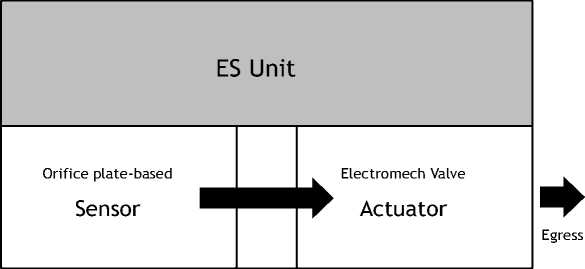
Water flow

Fig.6. Internal schematics of a Line Control Unit (LCU)

The typical operation of an LCU stems from the operation of an algorithm programmed into the ES unit. A flowchart illustrating this program is shown in fig.7. The potency of this control method is evaluated based on empirical data obtained from the experiment conducted with an LCU installed on a pipeline prototype shown in fig.2. The experiment data is presented in table 3.

Table 3. Sensor response delay test results

Leak Aperture (%)	Threshold: 200 KPa Response Delay (Min)	Threshold: 150 KPa Response Delay (Min)	Threshold: 100 KPa Response Delay (Min)
0	1000000.00	1000000.00	1000000.00
25	7.20	7.70	8.10
50	5.00	6.30	6.60
75	3.70	5.10	5.90
100	2.00	3.90	4.10

• 3.3.    Fault Control Experiment and Result

4.    Result Analysis and Discussion

• 4.1.    Water Production and Distribution Data Analysis

• 4.2.    Water Supply Infrastructure Fault Data Analysis

Fault control data of a pipe segment fitted with an LCU was collected in a real-time experiment using the research prototype presented in fig.2. The captured data describes the behavior of a typical pipe segment deployed in an expansive field implementation. Actuation control performance of the LCU is greatly dependent on its pressure sensor sensitivity threshold setting. This by design was set at 200KPa as the ideal threshold value hinging on prototype design conditions stated in section 2 of this work. The threshold was thereafter reduced in steps of 50KPa to observe the behavior of the sensor in terms of response time. It was observed that for different leak aperture sizes of the leak valve

(LV), different response delays occurred in minutes. These are shown in table 3 below. Analysis of the result obtained is presented in section 4.3.

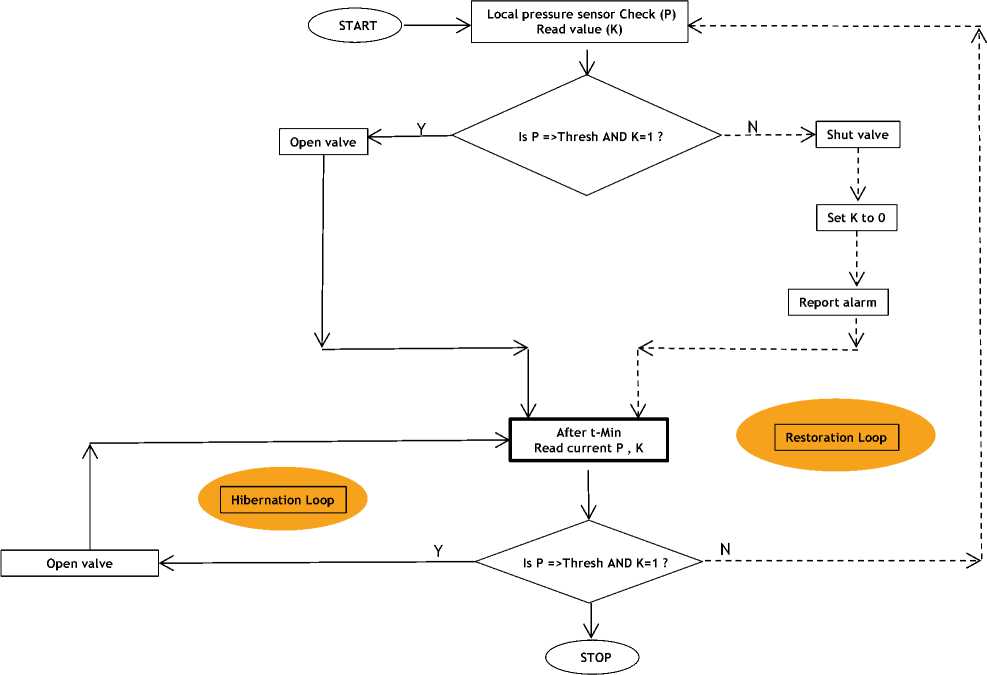
Fig.7. Operation program flow chart of an LCU microcontroller

This section presents analysis of the results obtained in this research and offers a comprehensive discussion of the findings made.

Fig.8 below shows the result obtained by plotting a linear regression graph for the bi-variate relationship between production and distribution loss based on field data tabulated in table 1. The graph in fig.8 shows a resulting linear relationship between the parameters, meaning that given other independent variables at play, distribution loss will increase in proportion with production quantity. Production quantity is budgeted to match consumption or utilization demand, however, if the causative factors of loss remain in place, distribution losses will vary in direct proportionality with production. This is a descriptive analysis of the production versus distribution loss behavior of the infrastructure under study, to provide insight into magnitude or order of the loss profile. To predict the future utilization profile of the water supply user-end, a Random Forest regressor machine learning algorithm was applied on the dataset presented in table 1. By this, a utilization model was derived to predict future utilization from end-users. The performance of this model was evaluated using the coefficient of determination (or R-square). The R-square value achieved was 0.93 or 93%. Based on the above information, it follows that performance prediction of supply utilization will be 93 per cent accurate with new data. Magnitude of loss profiled in the descriptive analysis in conjunction with utilization prediction capability provide useful insights cost-effective water treatment production and infrastructure maintenance planning.

The result obtained from the plot of MTBF and yearly failure rate from field data in table 2 is shown in fig.9. This descriptive analysis plot was achieved by use of linear regression machine learning algorithm. An approximate pattern generated by the algorithm is shown in fig.9, taking MTBF as the output or dependent variable and other features of the dataset as input or independent variables. Based on the graph in fig.9, the algorithm estimates by linear regression an inverse relationship between MTBF and failure rate per year. Meaning that going by historical data, as the number of failure rates rises due to incidences along pipelines the Mean Time Between Failures decreases. This bi-variate relationship exists between both parameters given the independent variable features listed on the failure data of table 2

as the driving factors. To predict the MTBF profile based on these driving factors in the dataset, a Random Forest regressor ML algorithm was used. The prediction performance was evaluated based on coefficient of determination (or R-square) metrics. The value obtained was 0.81 or 81% measure of prediction accuracy, meaning the prediction model will be 81 per cent accurate with new data. This prediction accuracy can be further improved using other ML algorithms in stand-alone mode or as hybrid of ML algorithm ensembled to achieve better prediction performance.

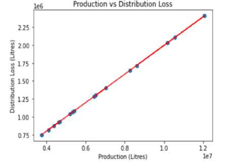
Fig.8. Distribution loss Vs production quantities fit

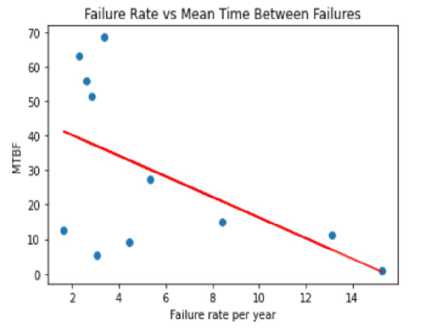
Fig.9. MTBF vs failure rate data line of fit

• 4.3.    Fault detection and Control Result Analysis

5.    Conclusions

Fig.10 and 11 present an analysis of the data tabulated in table 3. This analysis was done graphically using a python program to obtain the graphs represented below. The graphs obtained from the scenarios of observation show a decaying exponential behavior for the relationship between Leak aperture and Response delay for the given threshold pressure setting. With fine granular values of Leak apertures, the graph would come out as a smooth exponential decay curve, inflexing at a point between 20 and 30 percent of the full leak aperture size. These curves depict that shorter response delays under a normalized value of 0.2x10-5 minutes occur for Leak aperture sizes beyond 20% of leak calibration used in the design prototype, whereas smaller leak apertures below 20% of leak calibration result in longer delays before the leak is detected by the pressure sensor. Where there is no leak, meaning the leak aperture is 0%, the response delay tends to infinity ideally, meaning that no leak has been detected. This infinite delay condition is arbitrarily depicted by 106 on the data table above for illustrative purposes. Python programming tool used for analysis normalized all values on the Response delay axis to simplify the graph plot.

Interpreting the above result, it is fair to say that response delay of the pressure sensor device equipped on the prototype pipe segment LCU showed that for smaller leak apertures less than 20% of the full leak aperture size, there would be prolonged leak of water before the sensor detects the failure event and trigger the controller to drive valve closure actuation. From table 3, the highest empirical value for observed delay under a leak condition is 8.1 minutes and being that the leak aperture is small under this condition the amount of water loss is minimal prior to fault detection and control. In this case, it was only 17cl of water that was lost out of 15 liters in the supply tank, which is around 1% loss. Despite the empirical limitation of response delays, the system would still perform better than when left to leaks for days, months and perhaps indefinitely due to absence of maintenance intervention and automation of this nature, as is the case with most existing water supply infrastructure in developing cities in Nigeria.

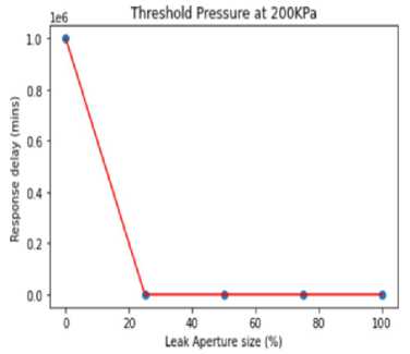
Fig.10. Response delay vs leak aperture for threshold pressure at 200Kpa

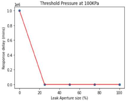
Fig.11. Response delay vs leak aperture for threshold pressure at 100Kpa

This research brings a proposition on the use of cost-effective solution leveraging a mix of embedded systems and Machine learning technologies for water infrastructure fault control, utilization data acquisition, processing, and forecasting for efficient water supply management. These indices are the core objectives and focus of this work. From control system programming, systems design, and dataset modeling using Linear and Random Forest regression ML models, it has been demonstrated that the operations of a water supply infrastructure can be modeled accurately from production to consumption stages, having reduced distribution losses caused by pipeline failures to the barest minimum using digital control schemes implementation. This research work brings a valuable contribution towards solving a key challenge faced in the supply of portable water through pipelines in most developing cities where government budget for infrastructure implementation and maintenance is minimal and investments are particularly low due to low returns and huge wastes of treated water in course of distribution via faulty pipelines. Deployment of such cost-effective solution along pipelines not only curb waste but also enable waterboard companies forecast accurately consumption profile of the user-end, hence determine appropriate production capacity per time. These together will boost availability of supply to end-users, revenue assurance to the production companies and thus encourage more investment into such infrastructure and business sector as consumption grows over time.

Acknowledgment

We acknowledge all contributing authors.