Discrete Wavelet Transform and Cross Bilateral Filter based Image Fusion

Published Online January 2017 in MECS

Nowadays, image fusion has gained much attention in image processing and computer vision. Image fusion is the process of combining the significant visual information from various source images of the same scene or view to produce a single enhanced image without any distortion or less information in images. The obtained fused image is more useful for human visual perception and further image processing operations [1]. Image fusion has been used in many disparate fields such as, medical imaging [2,3], military [4], surveillance [5], robotics and remote sensing [6], etc.

Generally, an image having less information does not provide an appropriate analysis of the scene. Consider, two images where one image is focused on some part of the scene and rest of part is in out-of-focus and another image is focused on the portion which is defocused in the first image however, defocused region which is focused in the first image. To get the entire scene in focus in a single image is a difficult task. Therefore, by integrating the relevant details from both the source images, a fused image with complete information can be obtained. This whole process of image fusion is called as multi-focus image fusion and these source images are known as multi-focus images.

The images captured from different sensors are multisensor images such as, CT (Computed Tomography) and MRI (Magnetic Resonance Imaging). These images may provide a different kind of information of the same organ to diagnose the diseases. CT images give the information of bone, blood vessels and hard tissues, whereas, MRI images give the information of the soft tissues. These two different images individually provide the different information according to their sensor ability but if we combined these images into a single image then all the relevant information (bone and soft tissues) of the organ can be presented in a single image which may provide more beneficiaries for diagnosis purpose. The fusion of multisensor images is known as the multisensor image fusion.

Image fusion process can be conducted at different levels, depending on represented information and applications. These levels are categorized into signal or pixel level, object or feature level and symbol or decision level [7]. In pixel level image fusion, the visual information of the source images is fused with their respective pixels to generate a single fused image. This level represents the lowest level of fusion. Feature level fusion defines the process of combining the features such as, edges, texture or color that have already been extracted from the source images. Finally, the decision level fusion represents the highest level of fusion, which combines the results from multiple algorithms to obtain a final fused image. Among these, pixel level fusion is widely used in most image fusion applications due to the advantage of containing original information, easy implementation and low time consumption.

Further, fusion methods can be categorized into two domains. One is the spatial domain based methods and the other is the transform domain based methods [11]. The spatial domain methods perform the fusion process in spatial domain directly. The spatial domain methods are time efficient and easy to implement. On the other hand, the transform domain based methods use transformations like, discrete wavelet transform [8], stationary wavelet transform [12], dual tree complex wavelet transform [13], and so on. Recently, some other transform domain based fusion methods are also introduced, such as curvelet transform [14], contourlet transform [15], nonsubsampled contourlet transform (NSCT) [16], multi-resolution singular value decomposition (MSVD) [17] and so on.

The pixel by pixel averaging is the simplest image fusion method and due to this it has attracted many researchers in the last decades [8-10]. But this method suffers from a number of undesirable effects, such as reduced contrast. To address this problem, multiresolution analysis based methods have been proposed, which consist of the following three basic steps. First, the source images are decomposed into multi-resolution representations with low and high frequency information and corresponding transformed coefficients are obtained. Second, the obtained transformed coefficients are combined together according to some fusion rules. Finally, the inverse transform is performed over the fused coefficients to reconstruct the fused image [18]. Generally, multi-resolution based methods provide better results than the other transform methods. However, the other transformations also preserve the same salient features such as edges and lines and are used in fusion. For an instance, a discrete cosine transform (DCT) based image fusion is introduced for fusion instead of pyramids or wavelet [19]. Again, a new multi-resolution DCT decomposition based image fusion approach has been given to reduce the computational complexity without any loss of image information [10].

Many image fusion techniques have been developed such as, maximum, minimum, average methods, principal component analysis (PCA) [26,30,31], intensity-hue-saturation [28]. In above discussed methods, average method provides the average information of the images but weighted average methods provide the information according to their weights and produce better fusion results. In [24], source images are fused by weighted average from the image details, where these details are extracted from the source images using CBF to improve the fusion performance. Hence, we proposed a novel pixel level image fusion scheme based on discrete wavelet transform and cross bilateral filter. The low frequency subbands are fused using pixel averaging method because approximation part contain most of the average information. Meanwhile, the high frequency subbands give the sharp details, therefore weighted average fusion rule is performed over the detail parts, where the weights of two different images contribute the information for fusion according to their weight value. The main contribution of this paper is to enhance the visual quality of the images by integrating all significant details of the source images using the pixel averaging and weighted average fusion rule.

The rest of this paper is organized as follows. In Section II, the basic theory of DWT and CBF are described. Proposed methodology is explained in Section III. Experimental results followed by discussion are presented in Section IV. Section V concludes the proposed work.

• II.    B ASIC T HEORIES OF DWT AND CBF

In this section, a brief review of the basic theories of discrete wavelet transform and cross bilateral filter is presented.

• A. Discrete Wavelet Transform

Discrete wavelet transform contains the multiresolution analysis property, therefore it is widely used in image processing. It converts an image from spatial domain to frequency domain   [8,27,20].  DWT decomposes the image into low and high frequency subbands. The low frequency subbands corresponds to approximation part, which contains average information of the entire image and is represented as (LL) subband. Whereas, the high frequency subbands are considered as detail parts containing the sharp information of images. The detail parts consist of three high frequency subbands (LH, HL and HH) as shown in Fig. 1 (a). For second level decomposition, only LL subband is further decomposed into four frequency subbands, whereas LH, HL and HH subbands remain as such, as given in Fig. 1 (b). The decomposition levels can be increased as per the requirement.

A 2-D DWT [20] for image f ( x , y ) of size m × n is defined as:

m - 1 n - 1

W _φ ( j ₀ , u , v ) =       ∑∑ f ( x , y ) φ _{j 0, u , v} ( x , y )  ⁽¹⁾

mn x = 0 y = 0

m - 1 n - 1

W _ψ ( j , u , v ) =       ∑∑ f ( x , y ) φ _{j , u , v} ( x , y )  (²)

mn x = 0 y = 0

where, Eqs. (1) and (2) are approximation and detail coefficients of image f(x, y) . Conversely, the image is reconstructed by performing inverse DWT. For the above given Eqs. (1) and (2), the inverse DWT is given as:

f ( x , y ) =    ¹   ∑∑ W _ϕ ( j ₀ , u , v ) ϕ _{j 0, u , v} ( x , y )

mn uv                   (3)

1∞

+      ∑ ∑∑ W _ψ ( j , u , v ) ψ _{j , u , v} ( x , y )

mn j = j 0 u v

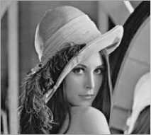
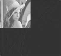
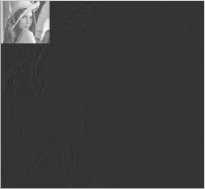
The DWT is applied over the image and the obtained results are shown in Fig. 2. Fig. 2 (a) shows the original lena image whereas, Fig. 2 (b) and 2 (c) show the first level decomposition and second level decomposition of the image after applying DWT.

LL1	HL1
LH1	HH1

(a)

LL2	hl2	HLi
lh2	HH2
LHi		HH1

(b)

location p is defined as:

X f ( p ) = i Z¹( li p - q II ) x G ®, ( i x ( p ) — x ( q )i ) x ( q ) ⁽⁴⁾

W qe 5

where , w = Z g^ (Ip - qG (Ix (p) - x (q) I) q e s

Fig.1. (a) First level DWT decomposition; (b) second level DWT decomposition.

(a)

is a normalization factor, || p - q || is the Euclidian distance between p and q.

Go (||p - qI) = e

III p ^- q I² 2 ^ 2

(b)

Fig.2. (a) Original lena image; (b) first level DWT decomposition; (c) second level DWT decomposition.

(c)

is a geometric closeness function and

_ I X ( p )- X ( q ) 2

Ga, (IX (p)—X (q )I) = e o

is a gray-level similarity or edge-stopping function. G os is a spatial Gaussian function that decreases symmetrically as the distance from the center increases.

G o

is also a Gaussian function that decreases with the

increase of the intensities difference between X(p) and X(q). s is a spatial neighborhood of the pixel p .

B. Cross Bilateral Filter

The Gaussian filter is the most popular filter which provides smoothness and removes noise present in the images. It is based on the weighted average of the intensity of the adjacent pixels. This filter removes the noise and provides smoothness but meantime also removes the sharp details. Therefore, to address this problem, the bilateral filter was introduced by Tomasi and Manduchi [21]. It is a local, nonlinear and noniterative filter which smoothes images while preserving edges and other sharp details. The bilateral filtering has been widely used in image processing applications. The spatial filter kernel is treated as a classical low pass filter used to obtain geometric closeness between the neighboring pixels, whereas the range filter kernel is treated like an edge-stopping function used for gray-level similarity between the neighboring pixels, which attenuates the filter kernel when the intensity differences between pixels are large. Both filter kernels are based on Gaussian distribution and the weights obtained from these filters depend not only on Euclidian distance but also on the distance in gray or color spaces. The bilateral filter (BF) is the combination of spatial and range filters [2224].

For an image X , the output of bilateral filter at a pixel

Parameters o  and  o are standard deviations of sr

Gaussian functions G and G   respectively and os             °T determine the amount of filtering for the image X.

Cross bilateral filter (CBF) considers both gray-level similarities and geometric closeness of neighboring pixels in image X to shape the filter kernel and filters the image Y . The output of CBF [24,25] for image Y at a pixel location p is calculated as:

Y cbf ( p ) = .1 Z G o ( II p - q II ) x G o ( I X ( p ) - X ( q ) I ) Y ( q )

W qe 5

where,

W = Z G o (I p - q|^G o (| X ( p ) - X ( q )) q e s

is a normalization factor and

l X ( p ) - X ( q )I²

Go (IX (p) - X (q )I) = e    2°'

is a gray-level similarity or edge-stopping function.

For images X and Y , the detail image is obtained by subtracting CBF output from their respective source

image and is given as X_D = X - X C _BF and Y_D = Y - Y C _BF , respectively. These detail images are used to find the weights by measuring the strength of details as reported in [24].

• III.    P ROPOSED M ETHEDOLOGY

In this section, we briefly discuss the proposed method. In the proposed method, two images having less information are used to produce a single composite image with enhanced visual quality. Here, the two source images either multi-focus or multisensor are used for fusion. The DWT is performed over both the source images to decompose the images into low and high frequency subbands. The low frequency subbands, which is also called approximation part, contains the average information of the images. The low frequency subbands of both of the transformed images are fused using pixel averaging method to get the overall average information from both the source image in a single fused image. On the other hand, the high frequency subbands are called detail parts which contain the information of edges and sharp changes. The high frequency subbands of both of the transformed images are fused according to their weights in respective images to get the sharp information in the fused image. Thus, the fused image has overall average information as well as dominant sharp information chosen from both the source images. The block diagram of the proposed method is shown in Fig. 3.

Low frequency subband

Pixel averaging based fusion

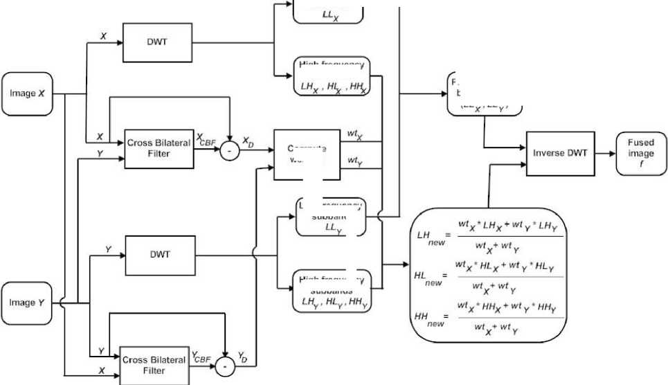
Fig.3. Block diagram of the proposed method

High frequency subbands

weights

Low frequency subband

High frequency subbands

The steps of the proposed method are summarized in Table 1.

• Table 1

Algorithm: Proposed fusion method

• 1.    Take two source images X and Y.

• 2.    Perform DWT over the images X and Y which decomposes the images into low and high frequency subbands.

• 3.    Apply pixel averaging method to fuse the low frequency subbands and obtain the average fused coefficient (LL new ).

• 4.    Combine high frequency subbands by their weighted average of both transformed images.

The weights are computed as in [24]:

• a)    Compute the covariance matrix as for both the images and then calculate horizontal and vertical detail strengths.

• b)    Integrate both detail strengths and obtain weight wt_X and wt_Y from images X and Y .

• c)    Fuse the high frequency subbands with their respective weights using:

• 5.    Perfom inverse DWT over the obtained fused coefficients ( LL new , LH new , HL new and HH new ) to reconstruct the fused image f .

  IV. E XPERIMENTAL R ESULTS AND D ISCUSSION

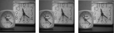
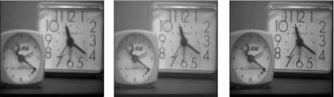
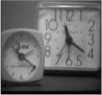
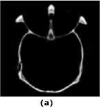
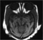
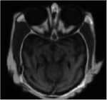
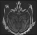
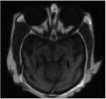
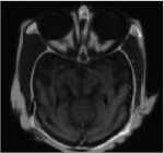
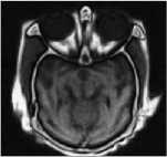
  The proposed method is carried out on several pairs of multi-focus and multisensor images as shown in Fig. 4, 5, 6, 7 and 8. Each image is size of 512 x 512 - Fig. 4 (a) and 4 (b) are blurred on left and right part images. Fig. 5 (a) and 5 (b) are upper side and lower side blurred images are called as dataset1. Fig. 6 (a) and 6 (b) are FLIR and LLTV images are called as dataset2. Dataset1 and dataset2 images are taken from [17]. Fig. 7 (a) and 7 (b) are hoed images which are blurred on middle and boundary part. CT and MRI images of size 256 x 256 are shown in Fig. 8 (a) and 8 (b) are acquired from the link The parameters o" =1.8 and ar =25 are used for the proposed method with window size 5x5 . The results of proposed methods are compared with some existing methods such as, DWT [8], PCA with DWT [26], SWT [12] and CBF [24] based fusion methods. The results obtained from above existing methods are shown in Fig. 4 (c-f), 5 (c-f), 6 (c-f), 7 (c-f) and 8 (c-f). However, the results obtained by proposed method are shown in Fig. 4 (g), 5 (g), 6 (g), 7 (g) and 8 (g). Visually it can be seen that in most of the cases, the fused images obtained from proposed method are better than other existing methods.

  But to evaluate the quality of fused image only visual inspection is not sufficient. Therefore, for quantitative measurement of the fused images some metrics are used. All the results of existing and proposed methods are tabulated in Table 2. It is found that in most of the cases the results of the proposed method have shown better performance than others and the best results are bolded. The metrics used in this paper are defined as:

  A. Average pixel intensity (API) or mean ( ц )

  It measures an index of contrast, which is defined as : mn

  YY f ( i , j )

  API =   ¹¹----- (7)

  mn

  
  

  £ Y (( f ( i , j ) - f ( i + 1, j ))² + ( f ( i , j ) - f ( i , j + 1))²)^V2

  AG = -^ j -------------------------------- ⁽⁹⁾

  mn

  
  

  D. Entropy (EN)

  It measures the amount of information presented in the fused image and is defined as:

  
  

  EN = - Y Pk ^log 2 ⁽ Pk ) k = 0

  
  
  
  

  where, p_k is the probability of intensity value k in image. The larger values denote better result.

  E. Mutual information (MI)

  It is defined as the sum of mutual information between source images and fused image and measures the degree of dependence of two images. The mutual information MI Xf between source image X and fused image f is given as follows:

  
  

  ^MIXf = Y ^hX ⁽ i , j ^)log 2 i , j

  
  

  h_Xf ( i , j ) h_X ( i ) h_f ( i , j )

  
  
  
  

  where , h_X f is the joint histogram between X and f , respectively. Similarly, MI_Y f represents the mutual information between source images Y and fused image f . The total mutual information between source images X, Y and fused image f is defined as:

  
  

  mi _tot= = MIx '+ MI_Yf total          Xf        Yf

  
  
  
  

  The higher MI_tota l value implies better fusion results.

  F. Fusion symmetry (FS)

  It indicates how much symmetrical information of the fused image with respect to source image and is given as:

  
  

  where, f(i, j) represents fused image and the size of image is m x n

  B. Standard deviation (SD)

  It is defined as:

  
  

  FS = 2 -

  
  

  MI Xf

  ^MItotal

  
  

  _-

  
  

  0.5

  
  
  
  

  SD =

  
  

  mn

  YY ( f ( i , j ) - ц )²

  i = 1 j = 1

  mn

  
  
  
  

  It reflects the spread in data and higher value represents better fusion result.

  C. Average gradient (AG)

  It measures a degree of clarity and sharpness and is defined as:

  
  

  G. Correlation coefficient (CC)

  It estimates a relevance of fused image to source image, larger value represents better fusion results which is defined as:

  
  

  CC = ( rX_f + rY_f )/2             (14)

  
  

  where,

  
  

  mn

  YY ( X ( i , j ) - x )( f ( i , j ) - Ц )

  
  

  i = 1 j = 1

  
  

  mn         mn

  YZ ( X ( i , j ) - X )² ZY ( f ( i , j ) - ц )² i = 1 j = 1                       A i = 1 j = 1

  
  

  and

  
  

wtx * HLX + wL * HLV

X  XY  Y

HLnew ------~----- wtx + wty

Similarly, we can obtain fused wavelet coefficients ( LH new and HH new ).

mn

ЕЕ ( Y ( i , j ) - Y )( f ( i , j ) - ^ )

i = 1 j = 1

mn         mn

ЕЕ (Y ( i , j ) - Y )² ЕЕ ( f ( i , j ) - д )² i = 1 j = 1                        JV i = 1 j = 1

(a)                      (b)                       (c)

• H.    Spatial frequency (SF)

It estimates the overall information level in the regions of an image and is calculated as:

(d)                         (e)                          (f)

SF = V RF ² + CF ²              (15)

where, RF and CF are row and column frequency

ЕЕ Е ( f ( i , j ) - f ( i , j - 1))²

RF =     --------------- mn

mn

ЕЕ (f (i, j) - f (i - 1, j ))2 izLJ;1------------------ mn

The large value of spatial frequency represents the large information in the image.

• I.    Q^XY/f

It evaluates the total information transferred from the source images to fused image [29]. Mathematically, it is defined as:

mn

Q^ = ЕЕ

[ Q X ( i , j ) w X ( i , j ) + Q Y ( i , j ) w Y ( i , j )]

ЕЕ ji [ w X ( . -. j ) + w Y (i, j )]

i =1 J =1

where, X, Y are source images and f is fused image. The definitions of Q^Xf and Q^Yf are same and given as:

Q X ( i . j ) = Q gX ( i . j ) • Q Xf ( i . j )

where Q^Xf ( i , j ) and Q^Xf ( i , j ) represent the edge strength and orientation values at location (i, j) , respectively. The dynamic range for Q^XY/f is [0,1] and it should be close to one for better fusion.

The other metrics L ^XY/f , N ^XY/f and N m ^XY/f are used to compute the total loss of information and noise or artifacts in fused image which are given in [9,24,29].

Fig.4. Fusion results for clock image: (a) left part blurred; (b) right part blurred; (c) fused image by DWT; (d) fused image by PCA; (e) fused image by SWT; (f) fused image by CBF; (g) fused image by proposed method.

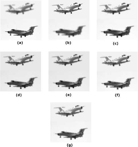
Fig.5. Fusion results for dataset 1: (a) upper part blurred; (b) lower part blurred; (c) fused image by DWT; (d) fused image by PCA; (e) fused image by SWT; (f) fused image CBF; (g) fused image by proposed method.

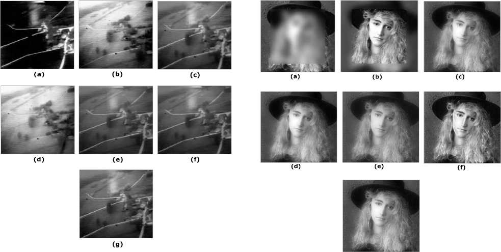
Fig.6. Fusion results for dataset 2: (a) FLIR image; (b) LLTV image; (c) fused image by DWT ; (d) fused image by PCA; (e) fused image by SWT; (f) fused image by CBF; (g) fused image by proposed method.

(g)

Fig.7. Fusion results for hoed image: (a) middle part blurred; (b) boundary part blurred; (c) fused image by DWT; (d) fused image by PCA; (e) fused image by SWT ; (f) fused image CBF; (g) fused image by proposed method.

Table 2. Image fusion performance measure

		Fusion metrics
Input Images	Fusion METHODS	SD	CC	API	AG	EN	MI	FS	SF	QXY/f	LXY/f	NXY/f	Nm XY/f
Clock	[8]	49.315	0.9721	97.038	3.879	3.8869	5.728	1.8904	6.2841	0.8341	0.1659	0.0017	0.0016
	[26]	49.315	0.9754	97.038	3.878	4.3445	5.875	1.8722	6.2817	0.8338	0.1662	0.0021	0.0013
	[12]	49.408	0.9872	97.038	4.471	4.4882	6.492	1.9021	7.4981	0.8700	0.1299	0.0118	0.0010
	[24]	49.892	0.9869	96.548	5.5265	7.2755	7.3415	1.9600	10.142	0.8982	0.0995	0.0114	0.0011
	Proposed	49.417	0.9890	97.080	4.4044	7.2761	6.8667	1.9934	8.0545	0.8583	0.1406	0.0155	0.0023
Dataset1	[8]	51.872	0.9746	221.43	3.1869	2.5333	5.0198	1.9587	10.2225	0.7958	0.2042	0.0296	0.0072
	[26]	51.873	0.9798	221.43	3.1871	2.8173	5.0368	1.9590	10.2232	0.7959	0.2041	0.0279	0.0079
	[12]	52.172	0.9876	221.43	4.2307	3.5672	5.3640	1.9526	13.5788	0.8698	0.1293	0.0036	0.0052
	[24]	52.561	0.9886	220.58	4.9215	4.2667	5.4154	1.9635	16.9262	0.9284	0.0635	0.0345	0.0081
	Proposed	55.242	0.9904	221.45	5.8073	4.7166	5.0230	1.9766	18.6560	0.8451	0.1473	0.0285	0.0076
Dataset2	[8]	40.394	0.5703	84.631	7.0495	1.9383	3.0799	1.7832	10.6120	0.6249	0.3751	0.0173	0.0036
	[26]	41.220	0.5770	84.631	9.7021	2.0432	3.0765	1.7704	21.9084	0.4599	0.5132	0.1035	0.1182
	[12]	41.087	0.5689	84.631	9.3246	2.0486	3.0832	1.7543	14.0195	0.7226	0.2753	0.0078	0.0065
	[24]	41.358	0.5317	84.665	9.7106	7.3465	3.0842	1.7735	16.8049	0.7305	0.2651	0.0184	0.0044
	Proposed	41.429	0.5815	86.642	7.7882	7.8537	3.4738	1.8188	17.4319	0.8310	0.1026	0.2124	0.0021
Hoed	[8]	56.559	0.9521	95.951	13.2480	1.9248	4.5982	1.8954	17.4967	0.7168	0.2832	0.0276	0.0028
	[26]	56.568	0.9460	95.951	13.2807	2.0431	4.7601	1.8643	17.5939	0.7188	0.2812	1.0231	0.0020
	[12]	57.947	0.9479	95.951	28.0801	7.6941	4.7803	1.8092	30.7982	0.8957	0.1007	0.0254	0.0036
	[24]	58.097	0.9628	95.958	22.8185	7.6988	4.6434	1.9987	30.9057	0.8775	0.1152	0.0626	0.0072
	Proposed	61.849	0.9566	96.173	25.2017	7.7399	6.9666	1.9952	33.9649	0.9478	0.0483	0.0226	0.0039
CT and MRI	[8]	34.883	0.6502	32.082	5.5005	1.6771	3.4601	1.6204	10.2717	0.6440	0.3560	0.0657	0.0110
	[26]	35.155	0.6521	32.082	6.6750	1.8607	3.4028	1.6082	13.1607	0.6140	0.3850	0.0052	0.0011
	[12]	35.107	0.6246	32.082	6.1676	2.0452	3.4122	1.6091	11.3466	0.6914	0.3086	1.5826	0.0021
	[24]	35.785	0.6905	32.166	7.2431	5.9698	3.4311	1.6554	14.7174	0.7143	0.2843	0.0065	0.0014
	Proposed	37.862	0.6545	41.414	11.5408	6.7736	5.5999	1.6122	21.0958	0.9116	0.0758	0.0873	0.0126

(d)

(g)

Fig.8. Fusion results for CT and MRI image: (a) CT image; (b) MRI image; (c) fused image by DWT; (d) fused image by PCA; (e) fused image by SWT; (f) fused image CBF; (g) fused image by proposed method.

• V. C ONCLUSIONS

In this paper, a fusion method of two multi-focus or multisensor images based on DWT and CBF algorithm is presented. In the proposed framework, the average and sharp details of the source images are integrated very cleverly into a single fused image. The performance of the proposed fusion method is tested against other fusion methods using several pairs of test images. Fusion performance is evaluated using many quantitative measurement criterions. Through the experimental results, it is found that the proposed method preserves more sharp information while eliminating artifacts and has shown better performance than other existing fusion methods visually as well as quantitatively.

A CKNOWLEDGMENTS

The authors would gratefully acknowledge the support of Dr. V.P. S. Naidu for providing us dataset1 and dataset2 for the test purpose.