Distributed Algorithms for Maximizing Lifetime of WSNs with Heterogeneity and Adjustable Sensing Range for Different Deployment Strategies

Published Online July 2013 in MECS

A wireless sensor networks (WSNs) is defined as a network of nodes that have small size and low-battery power and can be deployed to sense the environment for information collection. The collected information is sent through wireless links using multiple hops to a sink or controller, which can use it locally or further transmits to other networks through a gateway. A node in sensor network consists of CPU, memory, battery, and transceiver. The CPU performs data processing, memory stores data, battery provides energy, and the transceiver receives and sends data. The nodes can be stationary or mobile, location-aware or location-unaware, homogeneous or heterogeneous. The nodes in sensor networks can be individually addressable or group-addressable in which the aggregated data is communicated.

One of the important issues in sensor networks is power supply that is constrained by battery size, which normally cannot be enhanced. Thus, optimal use of the sensor energy has a great impact on the network lifetime [1]. This can be done either scheduling the sensor nodes to alternate between active and sleep mode or adjusting their sensing range [2]. The techniques that help enhance network lifetime can be either centralized or distributed. In former case, a single node has access to the entire network information that is used to determine scheduling. In the later case, a sensor can exchange information with its neighbors and that information is used to make scheduling decisions. The distributed algorithms require local (e.g., nearest neighbor) information due to limited memory, computing, and communication capabilities of the sensors. Scheduling is a very important aspect for the network lifetime. Paper [3] discusses a distributed algorithm based on using the faces of the graph. If all faces covered by a sensor are also covered by other sensors with higher battery level and these sensors are monitoring the region, then the first sensor goes into sleep state. This work has been extended in [4] and the resultant method is termed as the load balancing protocol (LBP). In this paper, they discuss maximizing sensor network lifetime for the given monitoring region using battery life and energy consumption rate for each sensor. Brinza and Zelikovsky [5] discuss how the sensors can interchange idle and active modes while monitoring and communicating. They discuss a new deterministic energy-efficient protocol for sensor networks (DEEPS) for prolonging the network lifetime. In [1,2,6], the network lifetime enhancement has been discussed by considering adjustable sensing range unlike the fixed sensing range in [4,5]. Papers [1,7] discuss a mechanism for making maximum disjoint covers sets of the sensors in such a way that one set can monitor all targets. These sets are randomly deployed to monitor the targets and have adjustable sensing range. The duration of the active set in [1] is energy dependent whereas in [7] all active sets have fixed time interval. The energy is conserved by activating the cover sets successively. The sensors from the current active set are responsible for monitoring all targets and transmitting the collected data to sink; and remaining go to sleep mode. In case a sensor is a member of multiple cover sets, such set covers leads to increase in the network lifetime. Paper [6] discusses the optimal scheduling by assigning the best times for each cover in order to maximizing the lifetime based on the ratio of number of uncovered targets covered by sensor and weight multiply by distance between sensor, and target of a target-covering sensor network. In [8], the network lifetime has been increased by constructing local cover sets consisting of sensors that can cover local targets. The cover sets are prioritized by using some properties of the lifetime dependency graph model. This work has been extended in [9] by enabling the sensors to determine their sleep-sense cycles based on specific coverage goals. In paper [10], a lifetime dependency (LD) graph model is discussed that captures the interdependencies between these cover sets by modeling each cover as a node and having the edges represent shared sensors. They also give some properties of the optimal schedule that relate to the LD graph into sleep-sense cycles. Paper [11] discusses the innovative models and heuristics by using exponential state space of the maximum lifetime sensor cover problem.

In [12], some mechanism is discussed to make sensors active. In this paper, the area left uncovered on removing a sensor is determined and it is termed as the sensing denomination (SD) of that sensor. Based on the location information of neighboring sensors, each sensor calculates its SD value in a distributed manner. The sensors with high SD have high probability of becoming active. If the cooperative nature of a sensor with its peers is considered, it leads to longer lifetime. This aspect has been addressed in [13] and named as multiple sensors to multiple targets (M-M) probabilistic target coverage problem. In M-M, multiple sensors cover multiple targets cooperatively and simultaneously with a given realistic detection probability threshold of each target. In [14,15,16], different deployments of sensors in 2-D are discussed, which include uniform arrangements in triangular, square, or hexagonal tiles and report that the triangular deployment is better as far as network lifetime is concerned. The network lifetime can be increased by providing energy heterogeneity to the sensors. The energy heterogeneity is addressed in [17,18,19]. These discuss 3-level heterogeneity models in which three types of sensor nodes: normal nodes, advance nodes and super nodes are considered. The advance nodes have more energy than the normal ones and the super nodes have more energy than the advance nodes. Their numbers are in reciprocal order because of the cost factor.

In this paper, we modify two distributed algorithms: deterministic energy efficient protocol with adjustable sensing range (ADEEPS) and load balancing protocol with adjusting sensing range (ALBPS) by incorporating 3-level energy heterogeneity. The resultant algorithms increase the network lifetime and are named as heterogeneous deterministic energy efficient protocol with adjustable sensing range (HADEEPS) and heterogeneous load balancing protocol with adjusting sensing range (HALBPS). Furthermore, the sensors are deployed in different tiles: triangular, square and hexagonal tiles similar to that discussed in [14-16]. The remaining paper is organized as follows. Section 2 discusses the network model. Section 3 discusses the proposed algorithms: HALBPS and HADEEPS. Simulation procedure is discussed in section 4. Section 5 discusses the results and the paper is concluded in section 6.

• II.    Network Model

In this section, we discuss different aspects of network model that include node types with their locations, their deployment strategies, and adjustable sensing range.

Consider N sensor nodes that are distributed randomly and uniformly over the monitoring field. We assume the following:

• •    It is a static and densely deployed network in 2-D.

• •    Each sensor node has information about its neighbouring sensors and targets, besides its own IDs and position.

• •    Each sensor nodes has adjustable sensing range and its transceiver has the capability to change transmission power for different transmission ranges.

• •    The sensor nodes are assumed of three types: normal, advance, and super nodes are considered like in [17

• 19]. The super nodes have maximum energy but reciprocal in numbers and the normal nodes have minimum energy; hence reciprocal in numbers.

• 2.1    Node Deployment Strategies

In this network model, the sensors are arranged in sets such that at any time only one cover set is active to monitor the environment and others are in sleep state to save the energy. The cover sets periodically become active according to monitoring schedule and that period is generally called reshuffle period.

Initially, the super nodes cover the targets. In case some targets are not covered by the super nodes, then some of the advance nodes that can monitor uncovered targets become active nodes. If some targets are still not covered by super and advance nodes, then some of the normal nodes that can monitor the uncovered targets become active nodes. The network lifetime is obtained by adding the times of each monitoring schedule. The network lifetime is increased using ALBPS and ADEEPS by incorporating energy heterogeneity and different deployments strategies.

The lifetime of a network is highly dependent on the nodes arrangement that in turn affects energy consumption in WSNs.

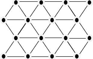
a) Triangular tiles

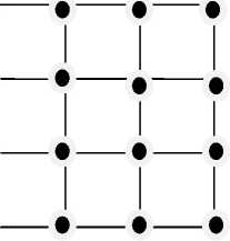
b) Square tiles

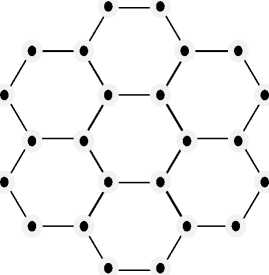
c) Hexagonal tiles

Fig. 1: uniform arrangement of the sensor nodes

There are several deployments/arrangements, but the most commonly used are triangle, square, and hexagonal in 2-dimensional region [14-16]. They are generally deployed manually by fixing the nodes in predefined locations to analyze for minimum energy consumption and hence the maximum lifetime of a WSN. Figs. 1(a)-(c) show deployment of sensor nodes in triangular, square, and hexagonal tiles [14-16].

• a) Triangle Deployment: In this deployment, the sensors are placed at each corner of a unilateral triangle. Each internal node shares 6 triangles at any point. We represent the area of a triangle in terms of the area of the exterior circle. The radius of the exterior circle d = √

• r, where r denotes the side length of the unilateral triang l e. The area of the network consisting of N nodes is N ^√ ; r² = N - ^√ - d² [14-16] (refer Fig. 2(a)).

• b)    Square Deployment: In this deployment, the sensors are placed at each corner of the square. The area covered by the network consisting of N nodes is given by 2Nd ², where d is the radius of exterior circle. (refer Fig. 2(b)).

• c)    Hexagon Deployment: A hexagon is a collection of six unilateral triangles as shown in Fig. 2(c). Each hexagon has 6 corners at which a sensor is deployed. The total area covered by N nodes is given by √3 Nd 2 (refer Fig. 2(c)).

  
  
  
  
  
  
  

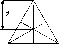
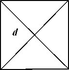
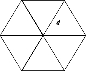
  Fig. 2: Coverage d, in triangular, square, hexagonal arrangement

  
  

• III. Proposed Work

• 3.1    HALBPS

• 3.2    HADEEPS

In this section, we discuss HALBPS and HADEEPS algorithms that are ALBPS and ADEEPS equipped with heterogeneity in sensor nodes. The sensor nodes are deployed in triangular, square, and hexagonal tiles. A sensor at any given point of time can be in one of the three states: active state, idle state, and deciding state. In active state, it monitors the targets and in idle state it listens to other sensors, but does not monitor targets. In deciding state, it monitors targets and will change its state to either active or idle soon. The characteristics of the HALBPS and HADEEPS are discussed in subsections 3.1 and 3.2, respectively.

This protocol is characterized by adjustable sensing range, deployment strategy, and node heterogeneity. With the help of load balancing, the HALBP is used to keep as many sensors alive as possible and try to let them die simultaneously. Here aliveness is different from activeness. Initially, each sensor disseminates its battery level and covered targets to its neighbors. It then stays in the deciding state with its maximum sensing range for finding sensor cover schedules. Each sensor will change its state as per following rules:

When a sensor is in the deciding state with range r , it will change its state to -

Active state with sensing range r , if there is a target at range r which is not covered by any other active or deciding sensors.

Deciding State , if all covered targets at range r are covered by either active or deciding sensors with a more prominent monitoring time. In that case, it decreases its sensing range to the next furthest away target.

Idle state, if the sensor decreases its range to zero.

First we divide the targets into sinks and hill. The hill target is identified by the energy accumulated from different sensors that can monitor it and has maximum energy. The remaining targets are sinks. There is one sensor-in-charge for each target besides that sensor monitoring it. The maximum lifetime of a target is defined in terms of sensor lifetime. It is the sum of the sensors’ lifetime, which cover that target. To determine the in-charge sensor of a target, following rules should be followed:

• •    For the sink target, the sensor covering it with the highest lifetime and the sink being the poorest target, is considered as the in-charge of that target.

• •    For the hill target, among the sensors covering the hill and the poorest target has the largest lifetime. Then that sensor is considered as the in-charge of that target. If there are several such sensors, the richest one is the in-charge.

The in-charge sensor remains active and others are in sleep mode. In order to find the sensor cover schedule, each sensor initially broadcasts its battery and targets covered to its neighbouring sensors in its range and then it stays in the deciding state with its maximum sensing range. Assuming the sensor in deciding state with sensing range r, it changes its state to:

• -    Active state with sensing range r , if there is a farthest target at range less than or equal to r which is not covered by any other active or deciding sensors.

• -    Idle state , whenever the sensor, not in-charge of any target except those already covered by the active sensors, switches itself to idle state.

For both the algorithms, the sensors make decision to go to active or idle state and stay in that state for a specified period of time, called shuffle time, or till the active sensor exhausts its energy. When the energy of an active sensor goes down below a threshold, it informs neighboring sensors and then goes to the deciding state with its maximum sensing range. A network will fail if there is a target which is not covered by any sensor.

• IV.    Simulation Parameters

We describe the parameters required to carry out them. Our methods: HALBPS and HADEEPS are simulated by deploying sensors in triangular, square, and hexagonal tiles. For simulation environments, a static wireless network of sensors and targets of 100Mx100M in which the sensors and targets are deployed randomly and their locations are known. We measure the network lifetime with respect to the number of sensors for different sensing ranges, numbers of targets using two energy models: linear and quadratic energy models. The parameters used in simulation are given in Table I.

Table 1: Simulation Parameters

Parameters	Symbols	Values
Number of Sensors	S	40 ~ 200
Number of Targets	T	25 and 50
Initial Energy of a normal Sensor	E0	2J
Adjustable Sensing Ranges	(r 1 , r 2 )	30M and 60M

The energies of a normal, advanced, and super node are assumed as E0, E0(1+ a), and Eo(1 + в, respectively, where a and в are positive real numbers. For taking total number of sensor nodes as n, the sum of the number of super and advanced nodes are given by n*m, where m is a positive fraction and the remaining n*(1-m) are normal nodes. Out of n*m nodes, n*m*m0 are super nodes, where is m0 a positive fraction, and the remaining  n*m*(1-m0) are advanced nodes. We employ two commonly used energy models: linear and quadratic energy model [18]. In linear model, the energy varies linearly with respect to distance and in the quadratic model, the energy varies quadratically with respect to distance. We have implemented the algorithms in C++.

• V.    Results and Discussions

We have considered two cases for analyzing the network lifetime using heterogeneity and different deployments in 2-D.

Case-I:       m=0.2, m0=0.5, α=2, β=1

Case- II:      m=0.2, m0=0.5, α=1, β=2

— ♦ —Triangular  — ■ —Square  —*— Hexagonal

No. of Sensors

(c)

Triangular        Square        Hexagonal

Triangular  — ■ —Square  —*— Hexagonal

No. of Sensors

No. of Sensors

(d)

(a)

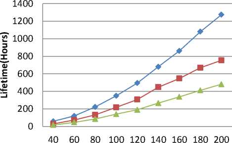
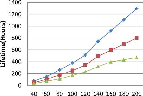
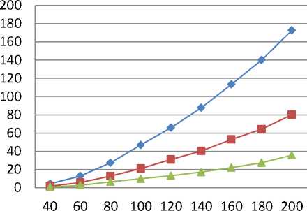
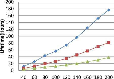
Fig. 4: lifetime for sensor networks in case of (a) HADEEPS with Linear Energy Model (b) HADEEPS with Quadratic Energy Model (c) HALBPS with Linear Energy Model (d) HALBPS with Quadratic Energy Model

Triangular  — ■ —Square

—*— Hexagonal

No. of Sensors

(b)

It is evident from these figures (Figs 4(a)-(d)) that as the number of sensors increases, the network lifetime also increases. It is intuitive because increasing the number of sensors increases the energy in network and hence network lifetime. The results further show comparison of network lifetime using triangular, square, and hexagonal deployment. We observe that the overall network lifetime significantly improves with both protocols for deploying sensors in triangular tiles for both linear and quadratic energy models. For using 200 sensors, the lifetimes obtained in the HADEEPS for deploying in triangular, square, and hexagonal tiles are 1296, 800, and 469, respectively, for linear energy model and, for quadratic energy model, are 176, 81, 38 hours. For same inputs and the HALBPS protocol, the network lifetimes are 1274, 753, 481 hours for linear energy model and for quadratic energy model are 172, 80, 35 hours. For other cases, the results are given in

Tables II and III for case-I and II, respectively. We observe from Tables-II and III that, in all cases, the results have similar nature.

Table 2: network lifetime using linear and quadratic energy models in HADEEPS and HALBPS for triangular, square, hexagonal deployments at different sensing range, different targets, and 200 sensors in 100M x 100M area for case-I

1.	Proposed Algorithms	Energy Model	Sensor Network Lifetime (in hours) at 200 Number of Sensor in hours
			Triangular tiles	Square tiles	Hexagonal tiles
	HADEEPS ( 30M Sensing Range & 25 Targets)	Linear	1296	800	469
		Quadratic	176	81	38
	HALBPS ( 30M Sensing Range & 25 Targets)	Linear	1274	753	481
		Quadratic	172	80	35
2.	HADEEPS ( 60M Sensing Range & 25 Targets)	Linear	1672	1072	646
		Quadratic	190	93	44
	HALBPS ( 60M Sensing Range & 25 Targets)	Linear	1491	988	631
		Quadratic	182	89	42
3.	HADEEPS ( 30M Sensing Range & 50 Targets)	Linear	975	607	357
		Quadratic	143	67	30
	HALBPS ( 30M Sensing Range & 50 Targets)	Linear	897	556	271
		Quadratic	104	42	14
4.	HADEEPS ( 60M Sensing Range & 50 Targets)	Linear	1134	739	488
		Quadratic	153	74	34
	HALBPS ( 60M Sensing Range & 50 Targets)	Linear	1011	695	447
		Quadratic	119	55	25

Table 3: network lifetime using linear and quadratic energy models in HADEEPS and HALBPS for triangular, square, hexagonal deployments at different sensing range, different targets, and 200 sensors in 100M x 100M area for case-II

1.	Proposed Algorithms	Energy Model	Sensor Network Lifetime at 200 Number of Sensor in hours
			Triangular tiles	Square tiles	Hexagonal tiles
	HADEEPS ( 30M Sensing Range & 25 Targets)	Linear	1208	748	439
		Quadratic	166	75	35
	HALBPS ( 30M Sensing Range & 25 Targets)	Linear	1189	703	448
		Quadratic	163	74	32
2.	HADEEPS ( 60M Sensing Range & 25 Targets)	Linear	1557	996	601
		Quadratic	179	85	41
	HALBPS ( 60M Sensing Range & 25 Targets)	Linear	1386	919	589
		Quadratic	170	82	39
3.	HADEEPS ( 30M Sensing Range & 50 Targets)	Linear	903	567	331
		Quadratic	133	63	28
	HALBPS ( 30M Sensing Range & 50 Targets)	Linear	838	518	252
		Quadratic	97	39	13
4.	HADEEPS ( 60M Sensing Range & 50 Targets)	Linear	1057	693	453
		Quadratic	143	69	32
	HALBPS ( 60M Sensing Range & 50 Targets)	Linear	937	649	420
		Quadratic	111	52	23

• VI.    Conclusions

In this paper, the energy heterogeneity in the sensor nodes and their deployment in 2-D in the form of triangular, square, and hexagonal have been discussed for both linear and quadratic energy models. The proposed methods - HADEEPS and HALBPS provide longest network lifetime for deploying sensors in triangular tiles for both energy models. The lifetime in case of triangular deployment is about two times more than that of the square deployment and three times more than that of the hexagonal deployment. Thus, in triangular deployment, the energy consumption has been found minimum.