Diversity Based on Entropy: A Novel Evaluation Criterion in Multi-objective Optimization Algorithm

Published Online September 2012 in MECS

Since Multi-objective Optimization algorithms has been a major concern in scientific field during the last decades, a number of performance metrics have been introduced to measure the performance of algorithms. However, there is unified definition and approaches for diversity performance measurement since a variety of diversity concepts are presented by different researchers. Apart from this, the existing assessment schemes have a limitation of individual solution’s dependence on its immediate neighbors [1].To make things even worse, the computational effort increases rapidly with the increasing number of solutions. Therefore, it is worthy of finding out an outstanding diversity metric in order to judging the efficiency and performance of algorithms.

In information theory, entropy is a measurement of the uncertainty associated with a random variable. In 2002, the entropy metric is introduced and highlighted by Ali Farhang-Mehr [2] in computing the diversity of Multi-objective Optimization Evolutionary Algorithms (MOEA). However, Ali Farhang-Mehr hasn’t clarified the detailed algorithm and the unified operation of the entropy metric. In Ali Farhang-Mehr’s paper, just several specific examples have been taken to explain the metric approach. That's to say, the effectiveness of entropy metric hasn’t been proved. Therefore, it’s quite difficult for us to choose the appropriate principle of entropy criteria operation when it comes to parameter and equation selection. Besides, further research deserves to be done since a great many of conclusions can be drawn with the help of entropy criteria. Tan K.C.’s has applied the Parzen window density estimation to estimate the probability density. While, K. C. Tan’s research [3] concentrates on Artificial Immune Algorithm and his entropy metric mainly relies on the concept of Antibody, which results in a limitation in application. Both the metrics mentioned above have been introduced to compare the efficiency of a specific kind of algorithm. There hasn’t been a unified entropy measurement experiment launched on different kind of Multi objective Optimization Algorithms yet, which can describe the diversity performance effetely and exactly.

In this paper, an entropy-based performance metric together with some key techniques such as appropriate selection principle and equation simplification are presented. A great many of experiments have been carried out to explore the diversity of different kinds of Multi-objective Optimization Algorithms, not only Multi-objective Evolutionary Algorithm but also Immune Algorithm. Experimental results have proved the efficiency and validity of the entropy metric on a quantitative basis. To some extent, this approach performs better in measuring the distribution of solutions in objective space. Firstly, we can clearly find out when to stop our optimization process. Secondly, with the help of entropy metric, we can figure out the algorithm efficiency on solving a specific kind of problems so as to select the suitable algorithm to optimize. Finally, we clearly find that the computational effort increases at a linear rate with the number of points in the solution set. Therefore, the further research about entropy metric will have a meaningful influence on how to preserve the diversity among different solution points of Multi-objective Optimization Algorithms.

The structure of the paper is as follows. Section II introduces the multi-objective evolutionary algorithm and the multi-objective immune algorithm. Section III states the diversity based on entropy, including Tan K.C.’s theory and Ali Farhang-Mehr’s method. Section IV presents the algorithm for diversity based on entropy together with the key techniques of entropy metric. In section V, a series of experiments have carried out to prove the effectiveness and validation of the entropy metric. Finally, we have reached our conclusions in section VI.

• II.    MOEA and MOIA

  • 2.1    Multi-objective Optimization Problem

Multi-objective optimization (MOP) has already been successfully adopted to engineering fields. In general, MOP consists of n decision variable parameters, k objective functions and m constraints [5]. Multiobjective Optimization [6] aims at conducting optimization for a range of functions as follows.

Maximize y=f(x) = (f 1 (x), f 2 (x) ,… , f k (x) )^T   (1)

Where x = (x₁, x₂, …. , x_m) ∈ Ω . x is called decision variables in the function. Ω is the feasible region in decision space ^[5] (or the definition domain of functions).

Let’s take maximization problem as an example, this kind of problem intends to achieve maximization for each objective. It is defined that a decision variable x A ∈ Ω dominates another variable x B ∈ Ω (written as x_A x_B) if and only if:

∀ i = 1,2,..., k , f i ( x A ) ≥ f i ( x B ) ∧∃ j = 1,2,..., k , f i ( x A ) > f i ( x B ) (2)

Then we define that a decision variable x* ∈ Ω is a Pareto optimal solution or non-dominated solution ^[5] if:

V x е П , x * >  x

Later, we define the Pareto-optimal set as:

P * □ { x * е П . З x е П , x ^ x *}

Generally speaking, the solution set is regarded as optimal when there are no solutions existing in the set, which is also called d Pareto front.

To sum up, to solve a Multi-objective optimization problem is to find out the pretty good Pareto- optimal front.

• 2.2    Evolutionary and Immune Algorithm

Multi-objective Evolutionary Algorithms (MOEAs) are an important research field when it comes to Evolutionary Computation. The overall purpose of the MOEAs is to organize, present, analysis, and extend existing MOEA research.

The Schaffer’s Vector Evaluated Genetic Algorithm [7], the Multi-objective Genetic Algorithm [8], NonDominated Sorting Genetic Algorithm (NSGA) [9] and Niched Pareto Genetic Algorithm [10] has the character of the first generation of Multi-objective optimization evolutionary algorithms, which adopt individual selection method based on Pareto ranking and fitness sharing to preserve the diversity among the population. The second generation of MOEA is presented from 1999 to 2002, including the Strength Pareto Evolutionary Algorithm (SPEA) [1], the Pareto Archived Evolution Strategy (PAES) [11], the updated vision Pareto Envelope-Based Selection Algorithm (PESA), PESAII [12], NSGAII and Micro-Genetic Algorithm.

Artificial Immune System is developed from biology immune system. It is a heuristic computing system designed to solve many kinds of difficult real problems based on the principle, functions, and basic characters of bio-immune systems. A lot of artificial immune algorithms have appeared recently, such as the MultiObjective immune system algorithm (MISA) [13], the I-PAES based on artificial operation [14], the Vector artificial immune system (VAIS) [15] and IDCMA [16]

• III.    Diversity Based on Entropy

  • 3.1    Existing Criteria about Diversity

Looking back on existing density assessments in measuring diversity, Goldberg's niche sharing, crowding density assessment, PESA, PAES, MGAMOO and DMOEA have been presented during the last several decades. Clustering analysis [10] has still been presented as an effective method in maintaining the diversity of the MOEA population.

Besides, several diversity performance criteria are introduced in detail as follows. Quality indicators are used to weight the result of the MOP problems’ quality, such as diversity, coverage and others. One of the most important quality indicators is Generation Distance (GD) [17], which measures the distance between true Pareto front and generated Pareto front. GD is defined as:

^N known

² known i                                (5)

i = 1

Where N known is the solution number of the generated front, and d i is the shortest Euclidean distance between each solution in generated front and the true front. The smaller GD is, the better the quality of the generated front.

Beside, Hyper-Volume Rate (HVR) [18] is also used as a quality indicator to measure the diversity of generated pareto-fronts. It is the Hyper-Volume Ratio of generated pareto-front and true front. The HyperVolume is defined as:

HV ( A ): = ∫ ₍ ⁽ ₀ ¹ _, ^, _, ^,1 ₀ ⁾ ₎ ∂ A ( z ) dz                           (6)

Where A is the objective vector, Z stands for objective space and ^∂ is the attainment equation.

Moreover, Inverted Generational Distance (IGD) is an “inverted” generational distance, in which we use as a reference the true Pareto front, and compare each of its elements with respect to the front produced by an algorithm.

j Z ⁽ d min ⁽ x , P ⁾⁾²

IGD ( p , p t ) =      ^{x ∈ pt}                                  (7)

| p_t |

Where Pt is the optimal Pareto solution set, P is the non-dominant solution set, dmin(x,p) is the shortest Euclidean distance between non-dominant solution x and the Pareto front.

However, these existing density assessments have some weak points to some extent. For example, the key to the niche sharing method is how to set a proper radius of the sharing parameter. The distribution is calculated by the number of solution sets. It’s hard to set and adjust the radius of the niche sharing parameter. In addition, the existing assessments always pay less attention to the exact diversity performance of Multiobjective optimization evolutionary algorithm measurement to some extent. Those algorithms never measure the distribution situation on a quantitative basis. Moreover, there are still fewer measures to preserve the diversity in evaluation process in a lot of evolutionary algorithms. What’s more, since there is no united definition of diversity for the reason that every researcher defines diversity in their performance metric. Therefore, it’s worthwhile to do further research on new diversity metric in order to measure the performance of MOEA at overall aspects.

• 3.2    Existing Diversity Based on Entropy

Looking back at previous researches, Tan K.C. and Ali Farhang-Mehr have ever presented relevant entropy-based metric.

Where K is the kernel function.

The multi-variate Gaussian kernel in the method is used and it can be described by

K ( Y ) = 1/(2π) ^{M /2}/( ∑ )^1/2exp( - 1/2* Y^T ∑^{- 1} Y )    (9)

Where R is the covariance matrix, T is the transpose operator, M is the number of objectives and the kernel width is defined by ^{σ = ∑ , σ ∈ R} .

uppbdj - lowbdj σj= archivebd

Where uppbd j and lowbd j denote the maximum and minimum values along the jth dimension of the feature space found in the archive respectively.

Entropy is defined in terms of probability density

I ( y i ) = - log( p y i )

As a result, the entropy-based density assessment can be summarized as

I ( yi ) = p ( yi ) ∑ ^1/2log( p ( y_i ) ∑ ^1/2)

• 3.3 .2 The Entropy Metric Proposed by Ali Farhang-Mehr

  Ali Farhang-Mehr presented his entropy metric in 2002 [2]. First of all, the objective space is divided into a series of grids. A function is defined to describe the influences among the solution points of population, which is called influence function. Different functions can be used as an influence function such as a parabolic function. What’s more, density function is applied to assess the density of the neighborhood information, which is defined as an aggregation of the influence functions of all solution points. After all the steps mentioned above, we can calculate the entropy value.

• 3.3    The Proposed Theoretical Entropy Approach

3.2.1 The Entropy Metric Proposed by Tan K.C.

Assume a stochastic process with n possible outcomes where the probability of the i-th outcome is pi. The probability distribution of this process can be shown as:

n

P = [ p 1 , p 2 ,..., p n ]; ∑ p_i = 1; p i ≥ 0;

^{i = 1}                                      (13)

In Tan K.C.’s general idea [3] is to make use of entropy to provide an estimation of the information content of each solution along the discovered Pareto front.

The Parzen window can be defined as follows [3].

This probability vector has an associated Shannon’s entropy, H, of the form:

n

H ( p ) =- ∑ p_i ln( p i ) i = 1

Where

pi ln(pi)

is assumed to be zero for pi = 0.

yi

P ( Y ) = 1/ Y ∑ K ( Y - y i ) i = 1

This function is at its maximum, Hmax= ln(n), when all probabilities have the same value, and at a minimum of zero when one component of the P-vector is 1 and the

rest of the entries in the P-vector are zero (Jessop, 1999). In fact, the Shannon’s entropy measures how evenly a set of numbers is spread [2].

Based on the previous work mentioned above, we have carried out a further research on the entropy metric. Generally speaking, we have master a lot of key techniques about the entropy measurement mention above after a series of scientific experiments. For example, the 3σ theory is introduced to calculate probability during the entropy measurement process. Besides, the appropriate parameter selection principle is proposed in order to reach an exact result. What’ more, we have simplify the density function in order to accelerate the optimization process.

Many metrics has never taken the actual distribution of the solution sets into consideration. Fortunately, the entropy metric mentioned above qualifies the combined uniformity and coverage of a Pareto Set [2]. In this case, the location of all solution points has already been under consideration. The result is a single scalar that reflects how much information a solution set transmits [2].

Since the core principle of entropy is to qualify the distribution of the solution sets based on the amounts of neighborhood information [4], the entropy metric can properly measure the diversity performance of Multiobjective optimization algorithms on a qualitative basis. To be more exactly, the entropy metric can quantitatively assess the distribution quality of a solution set in an evolutionary Multi-objective optimization algorithm.

The entropy metric is supposed to be an outstanding diversity performance metric from an overall aspect. In comparison studies of different optimization algorithms on testing one problem and the same algorithm on different problems, many conclusions can be drawn so that we can obtain a series of optimization suggestion. For example, the capability of the algorithms can be shown Apart from this, we can clearly find out the when to stop our optimization process since the entropy value remains constant which means the population of the solution set has reached its maturity. What's more, different algorithms have their own advantages in solving difference kinds of problems. As a result, we can select the most suitable algorithm to solve the specific problems. Last but not least, the computational effort of the entropy metric increases at a linear rate with the number of points in the solution set.

• IV.    Algorithm for Diversity Based on Entropy

  • 4.1    Entropy Metric Framework in MOA

When entropy metric is adopted to qualify the diversity performance of multi-objective optimization algorithms, we should pay attention to the position in which the entropy metric be added in the algorithm framework. Fig. 1 shows the flow chart of entropy metric in multi-objective optimization evolutionary algorithms, and Fig. 2 shows the one in multi-objective optimization immune algorithms.

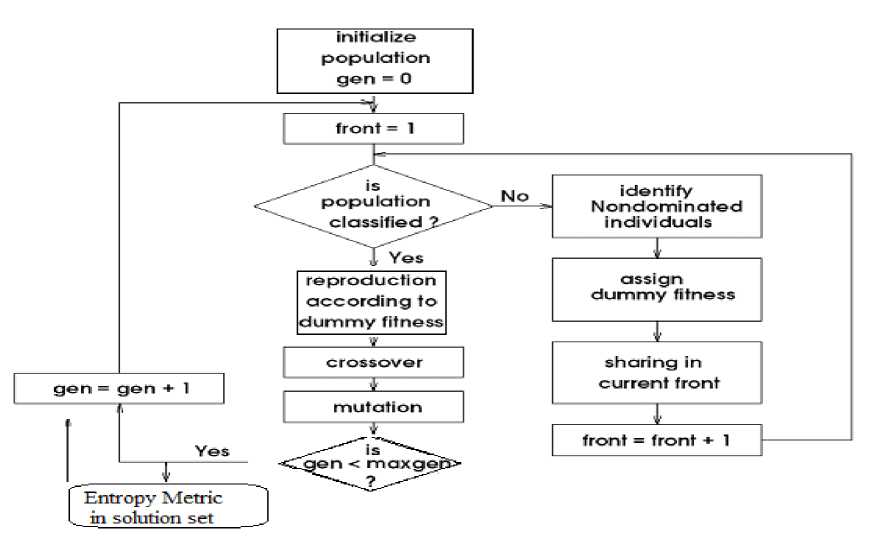
Fig. 1 The flow chart of entropy metric in MOEA

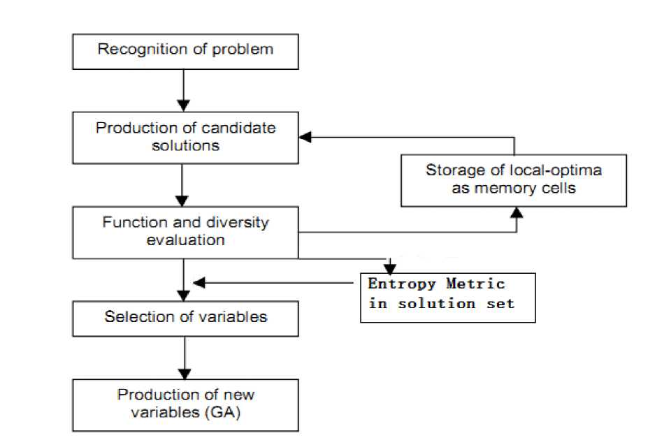
Fig. 2 The flow chart of entropy metric in MOIA

• 4.2    Entropy Computing Algorithm

Table 1 The Entropy Metric Algorithm

Set Algorithm parameters.

Initialize the relevant variables.

Obtain the maximum and minimum values of the Pareto front.

Get the normalized front and true Pareto front.

Divide the objective space into proper grids.

Adopt array to store the information in the grid.

Search for the dot in the grid.

• a.    Select a random point in the grid, and calculate its distance to other points.

• b.    Calculate the influence equation in objective space.

• c.    Calculate density function

• d.    Calculate the entropy of the whole solution sets.

In the last stage listed in table 1, the detailed steps are listed as follows.

Step1 Find out the necessary distance among the points in the grid.

The objective space can be divided into grids in order to calculate the entire information of the solution set. The grid division method adopted is to divide a certain length in every dimension on average. The principle of the grid method is to ensure the divided region become equal or less than an indifferent region. An indifference region is defined as the size of a cell wherein any two solution points within the region are considered to be the same or that the decision maker is indifferent to such solutions. Finally, we should find out the necessary distance among the points in the grid.

Step2 Calculate the influence equation in objective space.

The influence function defined here is Ω (li→y):R→R. Where r is the Euclidean distance between the i-th object and the y-th one. The standard deviation of this function is chosen subjectively according to the required resolution. The influence equation chosen in the paper is listed below.

^ ( r ) =

° 2 П * e ^{- (} r ⁾²

Where σ is the standard variance of distribution degree, and r is the space distances of the solution objects. We select the i-th object and calculate the value of influence equation between this one and other points.

Step3 Calculate the density function

The values for all points in the solution sets calculated from influence equation are collected after the traversal. It is easy for us to get the density value of every object after gaining values from the influence function. The object density is the aggregation of the influence functions between itself and all the other solution points.

na 1 a 2

D ⁽ y) = Z^{Q (} i^ ) ZE^{Q ( l (} <¹1,¹² > , y))        (16)

i = 1           ¹ y i = 1 i = 1

When it refers to m objects problem, the density function should be as follows.

na 1 a 2 am

D ( У ) 2 n ( l _ y ) = 2 2 -Z H ( l ( < 1 1, 1 2...

i = 1                              i = 1 i = 1        i = 1

^.. i m >  , У ) )

Where ^ ( ^l ( < i u ²^ i m > , У ) ) is the Euclidean distance between the i-th objective point and the y-th objective one in the a m –th dimension.

Step4 Calculate the entropy of the whole solution sets

We are supposed to calculate the entropy of solution sets according to the following equation. Since the sum of the entries (i.e., probabilities) in Shannon’s entropy definition is 1, we define a normalized density, ρ ij , as:

a ₁ a ₂

P ij = ^Dij/ 2 2 D k 1 D k ₂ k 1 ^{= 1    k} 2 = 1

Where D_i j can also be kept as D_i j (y) , which is the density function mentioned in step c. i and j stand for the position index in the grid, and the k1 and k 2 are the position index in the 2 dimension.

After defining the normalized density in the above paragraph, we can get the following equations:

a 1 a 2

2 2 p _k 1 k 2 ln( p k 1 k 2 ) = 1; p k 1 k 2 >  0; V k 1 k 2

k 1 = 1 k 2 = 1

wherein any two solution points within the region are considered to be the same or that the decision maker is indifferent to such solutions. Finally, we should find out the necessary distance among the points in the grid.

Let's mark the upper boundary it as lb k and the upper boundary as ub k (k=1,2…,r).Generally speaking, when it comes to a multi-objective optimization problem with r objectives, we mark the girds as (lb 1 ,lb 2 ,…,lb r ) and (ub₁,ub₂,…,ub_r).In addition, a grid can be divided into several little regions, which are called hyper-cubes(HC). The detailed division operation depends on the population of the evolutionary process and the number of objects that need to be optimized. Then, let’s represent the HC as r i , where i= (i 1 , i 2 , … ,i r ). Additionally, d represents the division times in every dimension, and d is a constant, larger than 2. Since the constant value of d is choosing subjectively, we should pay much attention to the principle of proper parameter selection. We are supposed to make sure that the size of every cell becomes less than or equal to a special region, wherein any two solution points within the cell are considered to be the same, or that the decision maker is indifferent to such solutions. As a result, the boundary of every r i can be described as

For a two-dimensional objective space, the entropy can be defined as:

rubk, j = [lbk + (ik I d)(ubk - lbk)] * wk

a 1 a 2

^H = - 2 2 P k 1 k 2 ^ln( p k'k 2 ) k 1 = 1 k 2 = 1

rlb k , i = [ lb k + (( i k - 1) I d )( ub k - lb k )] * w k

w k = range k I d

Generally speaking, for an m-dimensional objective space, where the feasible region is divided into a 1 *a 2 *…*a m cells, and the entropy of the solution sets can be defined as:

a 1 a 2 a m

• 4.3    The Key Techniques of Entropy Metric
  
  4.3.1    The Appropriate Principle of Grid Method

• 4.3.2    The Reasonable Parameter Selection

• 4.3.3    The Simplification of Density Function

We can see that the grid method has been adopted by many MOEA researchers in order to maintain the diversity of the evolutionary population. For instance, the grid method has already been introduced into PESA, PAES, MGAMOO and DMOEA algorithms, which has an outstanding performance in keeping the population diversity to some degree. Therefore, we have made the most of the gird method in the entropy metric with the intention of qualifying the neighborhood information as much as possible.

In terms of a multi-objective optimization problem with r objects, it is necessary to create a grid with 2r boundaries. The grid division method adopted is to divide a certain length in every dimension on average. The principle of the grid method is to ensure the divided region become equal or less than an indifferent region. An indifference region is defined as the size of a cell

Where ^{w k} is the width of every little region in the kth dimension and range k represents the width of the region.

The grid method provides the convenience of noting down the information of the solution sets and judging whether the point is in the grid or not. When it comes to m objects problem, we can create a super grid surface with ^{a 1* a 2*...* am} grids. We should pay enough attention that the number of super grid a 1* a 2*…* a m should be less than the evolutionary population. That’s to say, a 1* a 2*…* a m ≤ N.

The standard deviation of the influence equation is chosen subjectively according to the required resolution. In the equation, σ represents the standard variance of distribution degree. If σ is small, the changing rate of influence equation is very rapid. Therefore, it’s possible that the influence between the nearest points is too small to calculate. That’s to say, the density of the object can’t exactly reflect its distribution in the solution set. If σ is too large, this results in the stability of influence equation changing. It is hard to describe the point distribution via influence equation. Therefore, it is very important to select a proper parameter σ. In statistics, the three-sigma rule states that for a normal distribution when there are random errors during the process, nearly all values lie within 3 standard deviations [19] of the mean From the error analysis curve integral, we can see that more than 3 sigma appear error probability is very small. Therefore, three-sigma law has been proposed by many researchers, which says more than 3-sigma random error of data points should be abandoned. In other word, we choose 3σ theory to measure the information distribution in probability theory and random statistical theory. When executing the influence equation, we introduce the 3 sigma rule to get a proper value of 3σ. That's to say, we set 3σ equals to the range in the kth dimension. Therefore, the value calculated from the equation is more accuracy and reasonable.

As mentioned above, for two objects problem, we should use Equation (16) to calculate the object density. When it refers to m objects problem, the density function should be as Equation (17).

As a matter of fact, the density function can be simplified. The simplification principle is based on the assumption below. Generally speaking, we can choose b k = [(a k )^1/q].

Where q is an integer, which is no less than 2. Let b k =[(a_k) 1 ^/2].For a solution point yE F M whose corresponding super grid is 1, u2,… ,um>. Let ck = min{ u_k +b_k, a_k }, and d_k = max{ u_k –b_k, 1 }. Where u_k is the grid mark defined before. Therefore, the simple density function should be as equation 24.

D ⁽ У ) = I^{Q (} l i ^ y ) = I I-I ^{n (} l ⁽ < i i , i a,- , i m > , У)) (25) i = 1 i = d i I = d 2 i = d m

• V.    Experimental Results and Analysis

• 5.1    Test Problems, Test Algorithms and Parameters

• 5.2    Run time Analysis

We intend to evaluate the performance of MOEAs and MOIAs in producing adequate pressure for driving the evolution of individuals towards the Pareto front.

As Multi-objective optimization evolutionary algorithms, the non-dominated solutions distribute uniformly over the Pareto frontier. The evolutionary solutions cover the entire frontier during the period when the populations develop towards maturity. In this process, since the evolutionary population is on an increase, this definitely results in an increase in entropy. Therefore, when saturation takes place, the distribution quality improves a lot to some extent. That’s to say, the population becomes nearly all-feasible and nondominated, which spreads as uniformly as possible along the Pareto frontier. When it comes to the distribution situation, populations have already reached its maturity, at which point the entropy remains constant.

In order to evaluate the performance of algorithms in producing adequate pressure for driving the evolution of individuals towards the Pareto front, test problems we have chosen are Kursawe, DTLZI, ZDTI and ConstrEx problems. First of all, we give the detailed descriptions of test problems in the following table.

First of all, an experiment has been carried out in order to measure the execution time of using entropy metric as the quality indicator. Secondly, we choose a specific algorithm NSGAH to solve the test problem ZDT1.We note down the Pareto front and entropy value of the experiment in order to test the validity of entropy metric. Finally, we use entropy approach in measuring the performance of one algorithm in solving different optimization problems. The MOEA chosen are four kinds of Multi-objective evolutionary algorithms PESAII, SPEA, PAESn, NSGAH and two kinds of Multi-objective immune algorithms NNIA and MISA. The test problems are Kursawe, ZDT1, DTLZ1 and ConstrEx. What’s more, we compare MOEA using Entropy approach in measuring the performance of different algorithm in solving the same optimization problem.

An experiment of the execution time is carried out in order to analyze computing efforts of the entropy performance metric. The changes of execution time with the size of solutions increasing can be obviously observed in the following table.

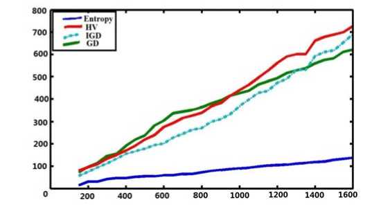
Fig. 3 The execution time of the evolutionary algorithm using different quality indicators

From the Fig. 3 above, we can clearly find out the computational effort increases at a linear rate with the number of points in the solution set. Take Sayin’s [20] metric for example, this is a kind of algorithm based on the distances of two points in the population and thus has a computational complexity of O (N2). Therefore, when it comes to dealing with quantities of data using diversity performance metric, entropy metric has an absolutely advantage over other metrics.

Ali Farhang-Mehr has explained that the density function of a solution set can be constructed and updated incrementally by choosing any new feasible solution point and aggregating its influence. Therefore, the less computing effort is an outstanding advantage of entropy metric in terms of diversity performance measurement.

• 5.3    Diversity Analysis

The entropy-based approach perfectly measures the distribution of the solutions in objective space, which exactly reflects not only the information of neighborhood solutions but also the whole solution sets in objective space. Data and graph are showed here to prove the validity.

Generally speaking, the population evolves towards maturity. The non-dominated solutions spread uniformly over the Pareto frontier which covers the entire frontier. In other word, there is an increase in the result of entropy. The entropy remains constant after the population has reached maturity.

Experiment 1: To test the validity of entropy metric

The experiment aims to test the changing situation of entropy with generation growing when it comes to solving different problems using single algorithm (the typical algorithm chosen here is NSGAII).

In this experiment, we have selected NSGAII algorithm to solving different problems. We have selected ZDT1, Kursawe, ConstrEx and DTLZ1 as the testing problems. In every group, we measure the value of entropy which is used as a quality indicator and the pareto front of the evolutionary process. The following graphs have shown our experimental results.

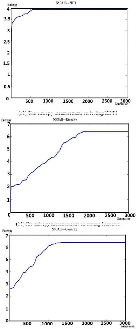
(a1) The entropy measurement on testing ZDT1

(b1)The entropy measurement on testing Kursawe

(c1) The entropy measurement on testing ConstrEx

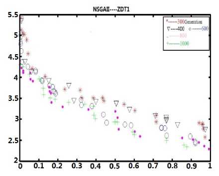
(a2) The pareto front on testing ZDT1

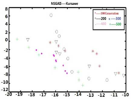
(b2)The pareto front on testing Kursawe

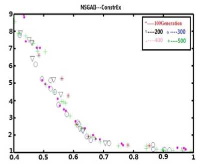
(c2) The pareto front on testing ConstrEx

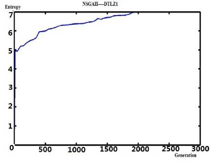
(d1)The entropy measurement on testing DTLZ1

Fig. 4 The entropy measurement and pareto front of NSGAII on test problems

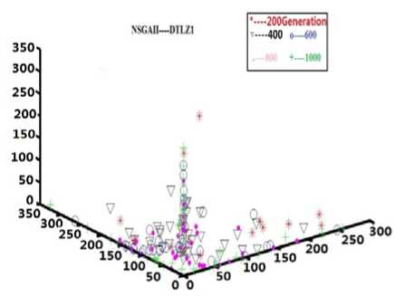
(d2) The pareto front on testing DTLZ1

As for NSGAII solving ZDT problem (shown in Fig.4 (a1) and Fig.4 (a2), it’s obvious that the entropy becomes a constant value and never changes when the evolutionary generation reaches 600. Compared with the situation of pareto front, the situation of evolutionary process improves a lot from generation 400 to generation 600. To tell in details, in (a1), the value of entropy is around 3.6 in generation 400.While, the entropy value reaches 4 in generation 600 and keeps constant after that point. In (a2), from generation 400 to generation 600, the diversity and convergence of solution set of the evolutionary process improves a lot. Therefore, it’s convinced that the entropy metric can be used as an effective quality indicator which reflects the diversity and convergence of the optimization evolutionary process.

Experiment 2: To Test same algorithm in solving different optimization problems

In this experiment, we intend to measure the situation of entropy when solving different problems using different algorithms. The diversity performance of two multi-objective Immune algorithms and four Multiobjective evolutionary algorithms are shown in the following graph. The detailed information about the specific experimental environment is listed in table 4.

Entropy is computed for every generation and plotted in the following graph in a similar fashion. We can draw a lot of conclusions from the experimental results.

We test the situation of entropy when solving different problems using different algorithms to compare MOEA using Entropy approach in measuring the performance of different algorithm in solving the same optimization problem.

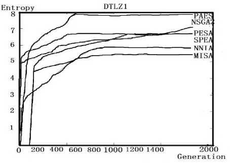
Form the following experimental results shown in Fig. 5, we can find that all the algorithms solve DTLZ problem at an efficiency rate. However, there are some differences which is worthy of paying enough attention to. Take PESA and SPEAII solving DTLZ as example, the entropy of PESAII have reached a constant value after generation 500, which the entropy of SPEAII has kept stable after generation 1200. As a result, we can draw a conclusion that we can select a specific optimization evolutionary algorithm to solving a specific kind of problems according to their efficiency of the evolutionary process for solving different kinds of problems.

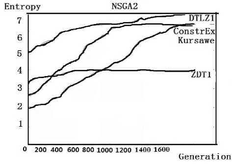
(a) NSGAII for different problems

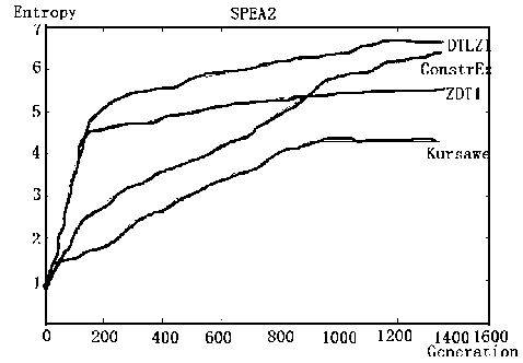
(b) SPEAII for different problems

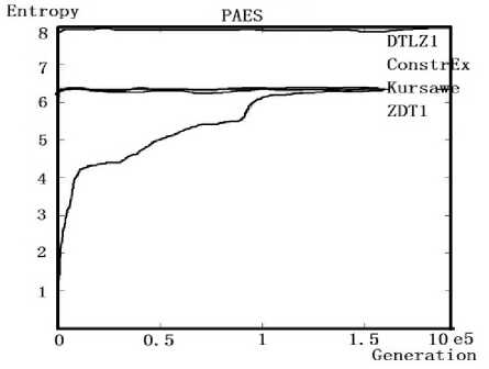
(c)PESA for different problems

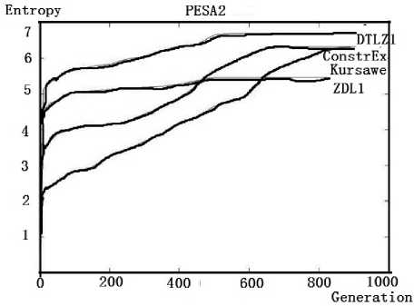
(d)PESAII for different problems

Fig. 5 Same algorithms for testing the different problems

Experiment 3: To Test different algorithm in solving the same optimization problem

Our experiment is to use entropy approach in measuring the performance of one algorithm in solving different optimization problem. We have the purpose of measuring the situation of entropy when solving same problems with different algorithms.

From the following graphs, we can find out different algorithms have their own advantages on testing different kinds of problems. For example, NSGAII have an outstanding performance on solving ZDT1 problem and does bad in solving ConstrEx problem while the performance of MISA is almost the same on testing different problem. As a result, we can select the most suitable algorithm to solve the specific problems.

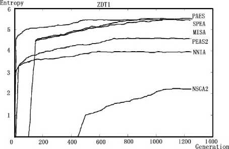
(a) ZDT1 problem

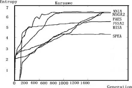
(b) Kursawe problem

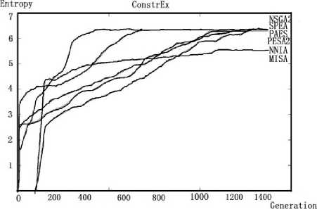
(c) ConstrEx problem

(d) DTLZ1 problem

Fig. 6 Different algorithms for testing the same problemIn comparison studies of different optimization algorithms on testing one problem, the capability of the algorithms can be shown on a qualitative basis. It is easy to find out the multi-objective immune algorithm can reach a constant entropy value at a quicker rate than other algorithms. That's to say, NNIA and MISA are two effective algorithms which can converge within a short time

Apart from this, we can clearly find out the when to stop our optimization process since the entropy value remains constant which means the population of the solution set has reached its maturity. Take the NNIA algorithm testing ZDT1 for example, the entropy value remains constant after the population reach 1000, at which point the population has reached maturity and we have already get well- distributed optimal solution sets. Let's carry out a further research using another index generational distance(GD).The following graph is the GD value captured during the process of NNIA algorithm on test ZDT1 problem. It's easy to figure out there is nearly no changes in generational distance after the generation reaching 1000. This is so called stopping point. In other word, the value of entropy keeps constant on reaching the stopping point and there is no need to continue the optimization process after the stopping point.

• VI.    Conclusion

This paper proposed a further study of the entropy metric presented by some researchers. The approaches of measuring diversity and the key techniques in programming based on entropy are presented. We have classified the appropriate principle of grid method, the reasonable parameter selection, and the simplification of density function in detailed.

As Multi-objective optimization algorithms, the nondominated solutions distribute uniformly over the Pareto frontier. In this process, since the evolutionary population is on an increase, this definitely results in an increase in entropy. Apart from this, we can clearly find out the when to stop our optimization process since the entropy value remains constant which means the population of the solution set has reached its maturity. It proves that the entropy metric have the capability of describing the diversity performance in evaluation process on a quantitative basis.

Some significant conclusions from the further study of this entropy metric are summarized. Moreover, the entropy metric has outstanding advantages over other performance metrics. For instance, the proposed entropy metric is of high efficiency in terms of computing since the computational effort increases linearly with the number of solutions. In addition, the entropy metric presented in this paper reflects how much information a solution set transmits about the actual shape of the observed Pareto frontier. That’s to say, the entropy metric have the capability of describing the diversity performance in evaluation process on a quantitative basis. What’s more, since the value of entropy stays constant when population of the solution set has reached its maturity, there is no need for us to continue our optimization work after the stopping point. That’s to say, we can define the right point in which the entropy stay steady as the stopping point. In other word, there is no need for us to continue our optimization work after that point.