DSGE-model for Russian economy with banks and firmspecific capital in coronavirus pandemic

Majority of dynamic stochastic general equilibrium models (DSGE) assume that the investments come from the households, because they hold the production factors. This assumption could, to some extent, be applied to the US economy where the households possess the company securities. However, the majority of the manufacturing and investment decisions are made by the managers of the American companies. We see this assumption to be inapplicable to the Russian reality. Taken this fact into account, we based our research on an understudied class of DSGE models (firmspecific capital) [1–3] which state that the firms make decisions concerning investment.

In the traditional DSGE models, the households practice direct investments, therefore, we need financial intermediaries who transform the household savings into the loans given to the real sector of economy. This is important to take into account as volatile periods could force the banks into rationalizing the loans in the real sector due to high risks rather than due to liquidity deficit. Along with that, the model accounts for the fact that the Russian companies invest their own resources into their fixed capital. Bank loans typically take no more than 25% of the investments.

The article describes the results of developing a DSGE model for Russia. Unlike the previous version of the model [4], behavior inertia is derived from the household behavior model rather than just declared ad hoc. The model also includes the investments into the fixed capital with inertia and a banking sector. Along with that, as it has been stated above, a firm-specific capital approach is applied to describe the investments.

The need to introduce the consumption and investment inertia into the model is determined by the following implications. Basic (inertia free) DSGE models demonstrate an immediate response to the exogenous shocks, while the empirical observations typically based on the econometric VAR models show hump-shaped response. Therefore, an inertia factor should be taken into account to improve DSGE models adequacy.

For simplification purposes, we consider the model free of budget and taxation policy of the state. Also for the sake of simplifying the reality, we take all investment goods to be imported.

In the view of the above, the purpose of the study is to construct a dynamic stochastic general equilibrium model for the Russian economy with a banking sector and the firms-specific capital under the COVIDcaused crisis.

Methodology and description of a

DSGE model

T he DSGE model describes the behavior of the following representative            agents:

households, real sector, financial intermediaries,

outside world, Central Bank. The Taylor equation describes the interest rate policy of the Bank of Russia under inflation targeting.

Household modeling

A representative household maximizes

the expected discounted CRRA (constant

relative risk aversion) utility function:

и = E

Y^

(

^(c t ^-h t ^{) 1} °~

1-^

—

1+p

Фь —+ ^L 1+p

.  —1-ф

+ Ф —-

^{+ Ф—} 1-^

)l

^ max ,

where Ep] is the operator of rational

expectations [5]; c_t is the consumption of goods and services; h_t is the variable showing the inertia of the consumer preferences (it will be further defined); L_t is the labour supply;

Mt mt = — is the real, while Mt is the nominal cash balances; P £ (0; 1) is the discounting rate for future utility.

A household budget constrains at t > 1 :

P t c t + M t + D t + D_w ,t = W t L t + M — +

+(1 + RD t- ₁)D t- ₁ + D w,t-i (1^^ ,  (2)

^ t-1

where P_t is the cost of living; D_t and D_wt are net assets of the households in the national and

foreign currencies with RD_t and RD_wt interest rates, respectively; W_t is the nominal wage; S_t is the nominal currency exchange rate.

The household budget constraint in real terms looks as follows:

^(ct + ^mt + d t + d w,t ^{— w}t^Lt⁾⁽¹ + nJ =

= m — + (1+ PD t-1 )d t-1 + d w,t-1(1+^^ ^^, (3) ^ t-1

where d = — and d = -^ are the real t    Pt         w,t     Pt assets in the national and foreign currencies; wt =Wt is the real wage; nt = pp— 1 is the consumer inflation.

Utility function (1) with the constraints (3) is maximized by the variables c_t,L_t,m_t,d_t,d_wt . The Lagrange function for the problem looks as follows:

L = E

- co i-'"Y:'  '

-1=0

-

1У41      mti ^\ фLТ+^ + ФmТ—ф)

—

—A t / (

(ct + mt + dt + d}

■ w,t

— W t L t )⁽1 + K t ) — m t-i

^—(1 + RD_t _1 )d_t -i - d w,t-i

(i+RD w,t-i )E t-i [S t \

S t-!

The first order condition for consumption is^ = /^(C t — У)^-а—А^(1 + K t ) = 0.

О C t

To define the adequate behavior of the households, it is necessary to specify the variable h_t . We will use the external habit formation model [6;  7]. This model

presupposes that h_t = hC_t-1, where C_t is some statistically average consumption driven by fashion or the accepted life standards. At the same time, there is an important assumption that the consumption of a particular household c_t cannot impact the macroeconomic variable C_t .

The received equation for the consumption c_t of a representative household gives the condition for the consumption C_t at a macroeconomic level:

(C t — hC t-i )^- ° = У(1 +К).              (4)

The first order condition for the labour

supply is ^ = —№_lL ’ + A t /^tW t ⁽1 + n t ) = OL t

= 0 ^ ФLL(pt = At(1 + njwt.(5)

For money demand-— = dmt

= /^tФ m m t ^- ^ — ^ t /^{t (} 1 + Kt) +

+ E[At+i]/t+1 = 0,(6)

^ Ф m m t ^ = A t⁽ 1 + K t ) — E[A t+i^] /.

For the deposits in national currency dL

= ^—A t ^/t(1 + ^Kt) +

@^d t

+E[A t ₊ i ]/^t+1(1 + RD t ) = 0,               (7)

E[A t₊i ]/ _ (1 + n)

^   A_t     (1 + RD t )

For the savings into foreign assets

A' -  +

+E[A_t+1]/^{t+i (i+RDw} , ^t)E[St+1] = 0,           (8)

S t

E^ t+AV _     (i+^ t )S t

A _t        (i+RDw,t)E[S t+1 ^]

Thus, under the equilibrium, the revenues of different assets should be equal ^(i+RDw A ) ^E[St+i \ = 1 + RD_t . The obtained ratio is the equation for uncovered interest parity (UIP):

E[S t+i] _   (i+RD t )

^St      ^(i+RDw,t )

Real sector modeling

As it has been mentioned above, we have described the situation when the firms make the decisions to invest into the fixed asset.

The firms are supposed to aim for maximizing the total discounted dividends to their owners once the investments are made: E 0 ^o =c /^t(1 —")n t ^max,                (10)

where P_{H t} is the prices of the national manufacturers; Y_t is the amount of the manufactured goods (actual GDP from manufacturing); cr_t is the amount of the bank loans at RK_t rate.

Manufacturing is described by the Cobb-Douglas function:

Y t = A t K t ^aL l ^-a,                           (12)

where A_t is the total factor productivity; K_t is the fixed capital stock. The dynamics of the latter is described by a standard equation with the investment adjustment costs:

^Kt ^{— K}t-i = ^It-i ^— P ^Kt-i ^— 2⁽T^{-1 — 1) I}t-1^{, (13) 2 l}t-2

where I_t-i is the investments into the fixed asset which are sourced from their own resources (from the profit share in the previous year) and bank loans:

P jt I t = шП t-1 +^cr t .                    (14)

Then, the Lagrange function for the manufacturer problem looks as follows:

£ = Е^ =оУ {(1 — ш)у — —X1 t (n t —P H,t A t KfLy^a + RK t cr t + W_tL_t) — ^— A2 t ( ^Pi,t^It ^— " ⁿ t-i ^{— cr}t ^{+ cr}t-i^{) — q}t ( ^Kt ^— —K_t -i (1 — ^—I - + ^ — 1)² It-i)]] .  (15)

The first order condition for the profit is: ^ = 0^Ay = 1 — u)+ o/E\A2_t+y (16) On t

The first order condition for the capital gives us the dynamics equation for the shadow price of the capital (the Tobin’s q ): d£ „        _   PHtYt        ____ ,

= 0^qt=A1ta —+(1 —ypE^t+il oKt                    Kt or in the real terms Qt = -^t-:

^P H,t

Q t =A1 t a^- + (1— ^)/E[Q t+i \(1 + E[K H,t+i ]) .  (17)

The first order condition for the investments is:

д£ „  _ „   _  _

— = 0^едл + Ш+1]^

дЦ

■(^-1)^

= ^,+2] 112:(^-1)-^.

or in the real terms:

A2 t ^pL+E[Q t₊i ](1 + £[^ H,t₊iD ^'

•Й-#^

= ш₊ 2 ](1+я[* _нл+1 ])-

• (1 + ^H,t+2D£2Z (^- 1)^.

Jt'4

We derive the labour demand from the first order condition for labour:

^£ = о^=(1-а)^.

OLt          PHr    4' L

We derive the equation connecting the Lagrange multipliers in the same way:

£ = 0 * ^2t = A1tRKt + /ЗЕ^+У(20)

о CT t

We assume that the real sector firms run in the context of the monopolistic competition. To derive the equation for the New Keynesian Phillips curve, we applied the Calvo price setting model [8].

We will refer to Gali and Gertler interpretation [9], who empirically proved that inflation data are better described with inflation inertia:

n_Ht = к mcr_Hi t + PE[n _H ,t+i\ + ^{(1 -} 0)^ —1 . ⁽²¹⁾

The real marginal costs will be derived from the following considerations. Let us assume that a representative firm has strategically developed its investment and manufacturing programs, as it has been described above. Operationally, they solved the task to minimize the costs subject to determined production volume. General costs are the solution to this problem¹ for the Cobb-Douglas manufacturing function: ^^Ш¹''’.       (22)

We calculate the real marginal costs dTC

MCR = -^, account for the manufacturer’s Ph , equilibrium conditions — = (1 - a) - and — = -a-L, and derive the expression for the —   1-aK’                r real marginal costs as:

mcr t = Y t -A t -(1- a)L_t - aKf      (23)

Foreign trade modeling

We have already assumed above that the investment demand is completely satisfied by the import. A consumer demand is shared between the domestic and imported goods. A consumer basket Ct contains domestic CH,t and imported CF,t commodities: в 1  в-1      1 в—1\в-1

C t = ((1-6 F y e C H ^e t +ау в с^\  .

Consumption maximization under the budget constraint  PH,tCHt + PFtCFt = PtCt gives the demand for the domestic goods:

— 6

CH,t = (1-8F)(-PH^)  Ct.(25)

and imported goods:

CF,t = 8F(pf)~e Ct.(26)

The equations above share

P = ((1-8yPH-e + eFPt-^f-i.(27)

the overall level of the consumer prices.

Similar to the equation of the demand for the domestic and imported goods, the external demand for the domestic goods is described as follows:

E t = Y c (/H-) * Y_w,f (28) ^ t ^P W,t

The global market defines the prices for the imported goods in a foreign currency. The law of one price works for the domestic market:

P F,t = S t P w,t ,                                (29)

P ,,t = S_tP wi,t -                                (30)

Modeling of financial intermediaries

We will follow the papers [10; 11] in modeling the financial intermediaries.

Loans to the firms in the real sector, holding the liquid assets in the Central Bank give the interest yield to the banks. The main expenditures include the deposit interest payments to the households.

To simplify, we do not account for the investments into securities and foreign currencies and do not explicitly allocate any reserves for the securities depreciation and possible non-performing loans. Therefore, banks maximize profit:

n _s,_t = R_tM_B , _t + RK_tcr_t - RD_tD_t -

-TC(D_t,cr_t) ^ max,                       (31)

where n _B,_t is the banks’ profit; M _B , _t is the liquid assets of the banks on the Central Bank accounts at the rate R_t ; TC(D_t,cr_t) is the operating expenditures from the assets management and deposit sourcing.

Balance of assets and liabilities is simplified as follows:

D_t + Cap_t = cr_t + M B,t + Res t ,            (32)

where Cap_t is the banks capital; Res_t is the banks obligatory reserves.

We assume that the banks capital is maintained on the minimally required level Cap_t = H • cr_t , where H is the capital adequacy ratio. The obligatory reserves in the Central Bank are Res_t = rr • D_t , where rr is the obligatory reserve ratio.

Then, the Lagrange function could be written as follows:

£ = R_tM Bt + RK t^ n - RD t D t - TC(D t , cr t ) --AB t (D t (1 - rr) - cr t (1 -H)- М в^ ).

The first order conditions for the liquid assets in the Central Bank are:

^a^^-w,, for the loans to the firms in the real sector:

^^=0^RKt = Rt(1-H)+^^^, dcrt                L       L for the household deposits:

^£=0^ RDt = Rt(1-rr)-^.(35)

dDt              t      t              gDt           47

For simplification purposes, we will further assume that marginal costs are constant.

Thus, the commercial banks set their deposit and loan rates on base of the Central Bank key interest rate. A business loan rate for the real sector goes up by the amount of the loan marginal costs which could include the loan risks, reserve sourcing costs, operating expenditures on loan administration. However, a deposit rate for individuals goes down if the monetary regulator increases the reserve ratio, and the marginal costs on the deposit sourcing grow. These rates determine the households’ decisions about their savings and the real sector firms’ decisions about their investments.

Now let us describe the results of the model linearization and its parameters calibration.

Linearization of a DSGE model and calibration of its parameters

To analyze the dynamic properties of the models in terms of deviations, we turn to the logarithms of the variables near their steady-state values (approximation of the percentage deviation of the variables from their equilibrium values)

X _t = ln ^ ; = lnX_t - 1ПХ * .

Log-linear approximation for the consumption gives

Ct = A£[Ct+i] + T^ct- -t 1+h

-rti^(RDt-E[nt+i]+n:T).

The consumption of the domestic and imported goods is

CLt = Ct + 9SFtott.

CF,t = Ct- drert,

p where RER = — is the actual currency p exchange rate;  tot = —  is  the trade conditions. Two variables are related by rert = (1- 8F)tott.(39)

Labour supply:

^Lt = Xt + (.п, - nT) + w,.(40)

Log-linear approximation for the marginal utility is

^■t = E[At+i] + (RDt -nt + nT).

Capital dynamics is

Kt = (1-p)Kt-i + pIt-i.(42)

Demand for labour is

Wt + SFtott = ?t- Lt.(43)

Investments are

• jt = i^^1,-1 + i+dl^^

^E[Q t+i] ^{+ E[n} H,t+i ^{] -}n^{T -}

⁺ х(1+Р⁽1+^ЕГ))

• -p^tUt+fiS).(44)

where Pit = —^ is the relative prices for the ,      PH,t investment goods.

A shadow price of the capital is

Q t = ^1^(^ t + Y t -E t' ) +

+ (1-p)l(E[Qt+i] + E\nH,t+i]  лТ).(45)

Stationary conditions for the real sector variables  are defined under the equations:  Л1 = 7----(1-^—, Q = Z Л1,

• 4           (i-a^i+^z^’ *’

Л2 = -^——,    RK = (1- |) ^,where

(1+nH)P P! ,          v^1^

aY_

1- ⁽ 1+n h ⁾⁽1—i⁾P К

Changes in the relative prices for the investment goods are defined by the equation1:

bp,,t = brert + nt- nHf(46)

Equations connecting the Lagrange multipliers dynamics in the firm’s problem are: ^t = ^^Zt,(47)

^t = (1- ^^t + RKt) + IE[^t+i].(48)

UIP equations with inertia at the foreign exchange market (for example, as a result of the enforcement of the budget rule): rer = ⁽ 1 - p RER^ Elrer t+i ] +

+P RER rer t-i + R™ - (RD t - E[n t+i] + л^Т). (49)

Dynamics of the prices on the imported goods is nFt = brer + л^(50)

Consumer inflation may be written as follows

Щ = (1 - ^F^Ht + ^f • KF.t.

Equation for export is

Et = ^tott + YWit.(52)

The Taylor equation for the key interest rate of the Central Bank is

R t = ⁽ 1- P R^n^t - л^{Т )} + q _y Y_t) + P r R -i . (53) Equation for the bank business loan and deposit rates is

RK_t = R_t+v_t,                          (54)

RD_t = R_t-v_t,                          (55)

where v_t is the shock of the marginal expenditures from the bank performance.

Equation for the output gap (a linearized macroeconomic identity):

^Y t = ^W CH ^C H,t + ^W E ^E t + AC t ,              ⁽⁵⁶⁾

where AC_t is the shock of the autonomous demand.

This obtained model is very similar to the classical Smets-Wouters model [12; 13], at least in the equations (36), (44), (45) describing the consumption and investment inertia.

As a result, the system (21), (23), (36) – (56) consists of 23 difference equations with the rational expectations and describes the dynamics of 23 endogenic variables.

For scenario simulations, the following shocks are defined in the model:

• -    total factor productivity;

• -    external demand, including global prices and oil production limits in OPEC+ deals;

• -    global interest rate;

• -    investments (for example, budget investments not explicitly defined in the model);

• -    total demand (for example, public procurements);

• -    inflation factor, besides the one described in the model (for example, changes in the tax rates);

• -    currency exchange rates (for example, country-specific risks triggered by the geopolitical instability);

• -    loan risks in the banking system.

Table gives the model parameters and their values calibrated under the data from Rosstat2 and the RF Central Bank3, as well as the estimates taken from other researchers [14–20].

The parameter | reveals a drawback of the calibration method⁴. Its value is calibrated closer to 1. As a result, NKPC equation shows a very weak inflation inertia that will be illustrated further in scenario simulations. This drawback is also manifested in a low impact of the interest rate on the investments. This is evidenced by the equation (48) connecting the capital return RK and the Lagrange multiplier A2_t , which is further included into the investment equation (44).

Parameters of a DSGE model for the economy of Russia Параметры DSGE-модели экономики России

Parameters	Value
Discount rate	£ = 0.996
Consumption inertia score	h = 0.7
Investment inertia score	Z = 1
Calvo parameter (inertia rate for domestic goods prices)	к = 0.56
Sensitivity of the key interest rate to inflation	<7 . = 4.40
Sensitivity of the key interest rate to output gap	q y = 0.13
Elasticity of intertemporal consumption substitution	о- = 0.12
Asset depreciation rate	/1 = 0.3
Capital elasticity of output	a = 0.7
Coefficient reversed to labor supply elasticity
Household consumption share in output gap	w E = 0.22
Export share in output gap	wE = 0.22
Import share in a consumer basket	SF = 0.44
Price elasticity of the domestic demand	в = 0.0786
Price elasticity of the external demand	£ = 0.0356
Share of re-invested profit	w = 0.5
Asset productivity in equilibrium	F к = 0.5 Л
Ratio of investment and consumer prices in equilibrium	Pi =100 PH

Thus, a DSGE model evaluated with the RF statistical data can be applied to analyze the economic strategy, as well as to evaluate the impact of different recessionary events on the Russian economy.

A DSGE model as an evaluation tool for the impact of the recessionary events on the economy of Russia

We apply the developed model to evaluate the impact of the latest recessionary events caused by the coronavirus pandemic on the Russian economy.

As a rule, calculations and impulse response function plotting consider an impact of every shock in isolation. In our case, different shocks affect the economy at the same time. Therefore, we defined single shock as an exogenous variable which was used in the equation with different coefficients. The following prerequisites were used as the multipliers:

• -    a 6% decrease of the external demand due to the global recession and OPEC+ deal;

• -    ruble depreciation by 15%;

• -    quarantine measures in manufacturing, services, as well as in international trade due to the coronavirus pandemic (–2% GDP);

• -    2.8 % GDP anti-recessionary measures (updated on 17.04.2020) with a 1 period delay.

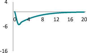
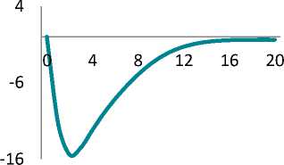
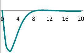
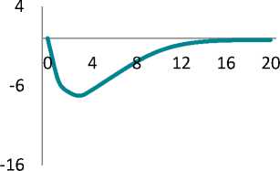
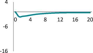
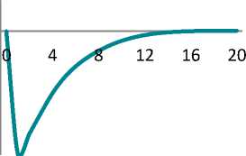
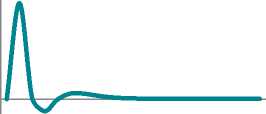
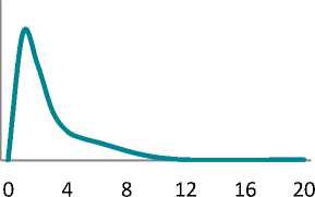
Figure shows impulse response functions illustrating a percentage deviation of the model’s key variables from their equilibrium values. Calculations were performed with Dynare 4.5.7 [21].

Russian labour market is known to be characterized by significant inertia. Our calculations show that a shock could be followed by a 2% decrease in employment. Population income and consumption could fall by 15%.

By the 2nd period, the investments fall by 15% and return to their equilibrium in 2 years. However, economy experiences longterm hangover of the under-investment: it takes 4 years for the fixed asset and 3.5 years for the labour productivity to gain their potential levels.

Inflation could accelerate by 2 percentage points, mainly due to the passthrough effect from ruble depreciation. In contrast, the prices for the domestic goods could experience pressure due to consumption reduction.

The maximum impact of the crisis on the output is seen in 3 quarters – a 7.2% fall in comparison with the before-crisis level. The impact of crisis is completely eliminated in 4 years only.

I

w

pi

R

-1

0    4    8    12   16   20

Y/L

-16

-6

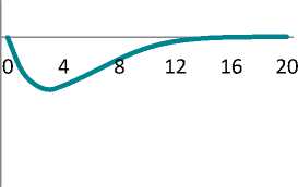
Impulse response functions for key variables (percentage deviation of the variables from their equilibrium values)

Функции отклика для ключевых переменных (процентное отклонение переменных от своих равновесных значений)

Let us apply the obtained evaluation of the crisis impacts to forecast GDP and inflation in Russia.

To do this, we should keep in mind, that in 2020, GDP could decrease less due to positive GDP dynamics in the 1st quarter (Rosstat estimates are not available), the trajectory of the potential economic growth (about 1.5%), as well as the additional measures of budget support and easing monetary policy. Our estimates for the economic recession in 2020 lie within the range from 5% to 7%. For 2021, the economic recovery is estimated to be within the range from 3% to 5%.

Inflation forecast should take into account the fact that the inflation is significantly below its target value (4%) in the previous year. The model forecasted that a short-term inflation surge could get the inflation figure close to its target value. With these prerequisites, the Central Bank could continue decreasing the key interest rate below a neutral level to boost the consumer prices.

The obtained results reveal, first of all, a dramatic scale of the possible recession in the Russian economy, which exceeds the 2015 crisis hangover and is comparable with the 2009 crisis. Secondly, the modeling findings evidence for a particular macroeconomic stability, in particular, the stability of the inflation processes in the economy of Russia. This differs the current situation from the previous recessionary episodes and makes a monetary stimulation from the bank of Russia with no outstanding inflation risks accessible.

Conclusion

The synthesis of the firmspecific capital approach and the prerequisites for possible investments sourced from the firm’s own resources in a DSGE model are the main theoretical outcome and the novelty of the research. This version of a DSGE model looks at low and negative interest rates at a different angle. As own assets are accumulated, a firm could experience a lower need in bank loans from large companies. What is more, these financial resources could compete with the bank loans, which decreases the interest rates. Equilibrium interest rates in DSGE models similar to the one described in this article are planned to be analyzed in further research.

A DSGE model is adjusted to the Russian realia and applied to project the trends in the national economy under the crisis caused by the coronavirus pandemic, which is seen to be the practical value of the research.

This model could be developed further into the specification of sector blocks and adding new elements. For example, the households could be divided into the Ricardian and non-Ricardian ones, the real sector could be divided by mining, manufacturing and investment goods producers. The model could also include the budget block which accounts for the impact of the taxes and public expenditures. Upon price setting modeling, an effect of the budget rule could be specified at the currency market. Finally, instead of calibration, the model parameters could be estimated by the Bayesian methods. All in all, this enhances the quality of a DSGE model as a predictive tool for making the political and managerial decisions.

Acknowledgements

The author thanks A.B. Polbin, the Deputy Head of the Macroeconomic Modeling Department in Gaidar Institute for Economic Policy for valuable comments and recommendations during the model development.