E-reputation prediction model in online social networks

Published Online November 2017 in MECS

Companies are nowadays aware that managing their reputation is crucial for improving their business. A good reputation can for example influence important stakeholder groups, employees and customers in global markets [1]. On the other hand, when a firm has a compromised image, its business is threatened, the sales may be impacted and customers may be reticent to deal with a company who has a tainted reputation.

Although reputation’s importance is undeniable for most marketers, its measurement remains the biggest barrier for an efficient brand management [2]. Being aware that social media are playing a key role in sharing opinions and that time is crucial in measuring reputation, companies are seeking for real time solutions that inform them constantly about their brand’s reputation as perceived by Internet users. Many Social Media Monitoring (SMM) tools are used for this purpose. They process a huge amount of content retrieved from social media channels and generate key insights about relevant messages, such as who sent them and when, what is their reach and what is the sentiment felt towards the brand. If SMM tools differ in terms of methods used and indicators highlighted, few score the reputation as a global value which can help the manager quantifying the reputation of its brand, following its evolution and comparing it with its competitors’ scores.

In literature, assessing reputation in a virtual community has been the subject of several works. Models proposed differ in how reputation is defined, which data is collected and which techniques are used. However, these models are mainly used in transactional environments like e-commerce or P2P applications [3] and where users are asked to score the product or to evaluate how trusty a member of the community is. In Social networks context, users are not asked directly to score a brand, they are instead expressing their feeling by message’s likes or dislikes, comments or shares, which leaves existing trust systems hardly applicable to these environments.

For scoring a global reputation in online social networks, we have developed an Intelligent Reputation Measuring System (IRMS) [4] that evaluates the reputation of a brand from the members’ activity - in terms of content posted or shared -, popularity and influence. However, this social information tends to change constantly. Thus, the reputation score can rapidly evolve. For this reason, we propose a reputation prediction model, based on propagation algorithms, which forecast the evolution of reputation score. We also assess the efficiency of proposed algorithms using real world social data.

The rest of the article is structured as follows: First, we give an overview about the background and related work. Second, we present the Intelligent Reputation Measuring System. Then, we focus on the prediction model and present proposed algorithms. Experimentation of the system is discussed in the following section. Finally, we conclude with future axes of our work.

• II.    R elated W orks

Reputation has been the subject of several works which designed different models of trust systems. These systems aim to measure reputation in virtual communities according to the nature of the social network and to the definition given to reputation which is confused most of the time with trust. Trust, according to sociologists is “a bet about the future contingent actions of the trustee” [5]. In other words, Trust is linked to actions expected from the trustee toward the trusted. This definition is also used in some works in computer science field where trust is defined as: “a subjective expectation an entity has about another’s future behavior” [6]. Although trust and reputation are semantically close in most cases, a difference is noticeable in Ref. [7] where reputation is described as: “the aggregated perception that an agent creates through past actions about its intentions and norms”. Thereby, unlike trust which is a one to one relationship, reputation is considered as a many to one relationship. This inspires the definition we give to reputation in IRMS model.

Definition : Reputation is the amount of estimation in which an entity is held by the community, based on information and experience shared.

In literature, several models of reputation systems exist. They differ in what information is collected, how information is processed, who intervene in this process and where reputation is measured. In a previous work [4], we proposed a taxonomy of reputation systems which we modeled under five dimensions:

• 1)    The “what”, describing the type of collected data. In social networks, available information belongs to, either users’ activity or popularity. Activity in turn can be further classified into two types of information that are opinions and popularity.

• a.    Opinions expressed by a user in the community can either be a direct rating like in e-commerce communities, or a message added like articles shared, comments posted, content approved or disapproved, etc. As to interactions, they concern the behavior of the user in terms of the number of messages sent, their duration or frequency. Examples of interaction based trust systems can be found in Ref. [5]

• b.    Popularity, which shows how famous a user can be in his community, can also reveal useful information to trust systems concerning the

number of neighbors that can read messages sent by each user and trust them [8].

• 2)    The “How”, indicating reputation assessing techniques. These techniques vary between statistics, machine learning and heuristics. One of the most frequently used statistical methods is the Bayesian Model [9]. As a statistical technique, Belief theory is also largely used in some trust systems [5]. In the Belief model, trust is based on the user’s belief in the trustworthiness of a rating statement. Artificial Neural Networks (ANNs) and Hidden Markov Models (HMMs) are machine learning techniques used in some trust systems. As an example of trust systems using ANN, Ref. [10] proposes a brokerassisting information collection strategy based on clustering method.

Instead of complex statistical or machine learning solutions, many researchers have chosen heuristics based solutions for computing and predicting trust. For instance, Ref. [11] proposes a robust trust system based on an easy to construct and to understand method.

• 3)    The “Who”, is defining peers considered in computing trust which can either be a global or a local metric. While global trust is based on complete graph information and is considering all peers in the network, the local trust is computed using partial graph information and taking into account personal opinions. Some examples of systems based on global or local trust metric are referenced in Ref. [12].

• 4)    The “Where” is the spatial dimension defining the environment where trust systems operate. Many reputation models are developed in virtual communities such as e-commerce systems, distributed applications, social communities, etc. Social networks, on which our research is focused, are sharing some common properties such as the graph based structure where nodes refer to the community members and edges to their relationships. Processing these large graphs needs often sophisticated techniques for social network analysis [13]. Relationships are supposed to reflect homophily , which is the members’ tendency to create relationships with individuals sharing the same affinity according to their social status or personal values.

• 5)    The “When”, as its name indicates, is the temporal dimension. Being aware that reputation is vulnerable to time, many researchers have introduced the forgetting factor in their Reputation systems [14].

• III.    I ntelligent R eputation M easuring S ystem

• A.    Reputation Model in IRMS

When marketers or companies’ managers are monitoring their reputation in an online social network, they are seeking an indicator that allows them to measure their brand’s reputation as perceived by members in that community. In IRMS, reputation is global and representative of the common perception held by the network members who have expressed an opinion about the brand or have received feedbacks from their relationships. Hence, the reputation measured by IRMS is also people centric since it is composed of local one to one reputations that are perceived by each member concerned.

Furthermore, the opinion expressed by a user in the social network can differ according to the context concerned, and the appreciation of the product in other contexts may be different or even opposite. For instance, a smartphone may be appreciated for its design but may leave users less enthusiastic regarding its features. Considering this context dependence, IRMS structures reputation as a vector whose coordinates represent reputations associated to each context or relevant attribute of the product evaluated.

Let N be the number of contexts related to the product or the brand for which we want to measure reputation, and rk ∈ [0,1] the reputation corresponding to the context k . Reputation measured by IRMS is modeled by:

( ^1 ^, ^2 ,…, ’n ).

Thereby, we define the reputation of an object O according to a user U as the magnitude of the vector ⃗⃗⃗⃗⃗⃗⃗⃗⃗⃗⃗ _:

Repu = ||^{⃗⃗⃗⃗⃗⃗⃗⃗⃗⃗⃗⃗}|| = √ ^ri + ^T2 + ...+ r^ . (2)

If we take back the example of the smartphone, each specification like design, display, camera, hardware, connectivity, features, etc., can be associated to a context. Since contexts may not have the same importance – the color of the smartphone for instance may be less important than its features-, IRMS attributes weights to each context according to its impact on reputation:

||^{⃗⃗⃗⃗⃗⃗⃗⃗⃗⃗⃗⃗}|| = √ ^wi^ri + ^W2^r2 + ...+ W^N (3)

where wk ∈ [0,1] is the weight of the context k . Hence, when all mono context reputations rk are null, reputation Rep^ is minimum, and when all the coordinates rk are equal to one, Repu is maximum. To range the reputation score in the interval [0,1] and facilitate results interpretation for IR MS u sers, we normalize the magnitude of the vector :

Repu

||⃗⃗⃗⃗⃗⃗⃗⃗⃗⃗⃗⃗⃗⃗||

√W^ + W2 + ⋯

√ w?r?+    +

√        ⋯

√W^+ W2 +⋯

To define the mono context reputation rk we use the Beta probability density function of the Bayesian model. This method is suitable for representing probability distributions of binary events [15], which are in our case, the advent of positive and negative opinions (Note that a neutral message can be substituted by a tuple of positive and negative opinions).

Let (p, n) be respectively the amount of positive and negative messages expressed by a user U in the social network concerning a context ck of an object O for which we are calculating the reputation score. The reputation of O as perceived by the user U according to the context ck is represented in the form of the probability expectation value of the beta PDF:

=

Pc_k + 1 P^_k+n^_k

As the global reputation score measured by IRMS is people centric, it is obtained by averaging reputation scores of the object O as perceived by each member in the social network who has a direct or indirect experience with O. This group of users is called the Group of Reach and is composed of active users who have expressed an opinion in the network about the object O , and passive users who have received the feedback of their friends and eventually have been influenced by their opinions but did not react in their community.

• B.    Reputation Measurement Processing

Unlike many reputation systems which base their calculations on ratings, IRMS considers useful data in the network and collects opinions posted by the community members about the object O. For the sake of simplification, old messages are ignored and recent messages are processed in order to learn, for each message caught, the user who send it, the polarity of the opinion expressed, the context of the message and the time when the message is posted. To extract this information, we can use techniques of opinion mining and sentiment analysis [16]. This data is then taken as input in the form of the tuple < user, opinion, context , time>. IRMS uses also the graph structure of the network to learn the neighbors of each active user.

Once messages are collected and useful data is extracted, IRMS is ready to process the reputation measurement which is undertaken in five steps as illustrated in Fig.1. :

• 1)    Step (a): Learning local context specific reputation. Based on the Beta Probability Density Function, IRMS computes for each context, the reputation of the object O as perceived by any user U who has expressed on opinion about O in the network

• 2)    Step (b): calculating reputation score for active users. In this step, IRMS calculates the local reputation, for each user in the matrix of mono context reputation, using its corresponding coordinates r _k according to (4). Weights w _k are configurable in IRMS and can either be preset by the system user or suggested by a machine learning system. Note that users in the matrix of step (a) are the whole active users belonging to the Group of Reach

• 3)    Step (c): Defining the Group of Reach. Active users being already identified in step (a) and (b), the Group of Reach is completed with its passive neighbors who could be influenced by their active friends even if they did not react in the network. IRMS extract passive neighbors from the graphical structure of the network and retains

the passive ones since active neighbor are already counted in previous steps

• 4)    Step (d): Deducing reputation score for passive neighbors. A member in the social network who has one or more active users is influenced by his friends’ opinions as he is sharing affinity with them. The local reputation of the object O as perceived by a passive user P N is the mean of reputation score of his active neighbors, attenuated by an influence degree θ ∈ [0,1] which depends on the nature of relationships in the network:

Rep _ score^PN =θ ^∑ Nb of act _       _               (6)

^_                         Nb of act _

• 5)    Step (e): Computing the global reputation score. The global reputation score of the object O is the average of local reputation scores of all members of the group of reach:

Global Rep score = ^∑ Rep _ reUser^ ∑ Rep _ :ore^PNk (7) || groupe of reach. ||

The efficiency of IRMS has been experimented using real world social data [17].

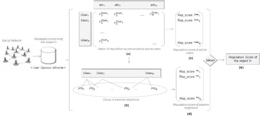
Fig.1. Processing steps of reputation measurement by IRMS

• IV.    R eputation P ropagation in S ocial N etworks

The reputation score of IRMS is based on past information pouring in the system. The result is updated each time new messages are created in the social network. Thus, the IRMS score measures an instant reputation and doesn’t inform the user about the evolution of this metric in the future. For this purpose, we propose an enhanced algorithm that measures reputation using forecasted messages propagation in the network.

• V.    R eputation P ropagation in S ocial N etworks

The reputation score of IRMS is based on past information pouring in the system. The result is updated each time new messages are created in the social network. Thus, the IRMS score measures an instant reputation and doesn’t inform the user about the evolution of this metric in the future. For this purpose, we propose an enhanced algorithm that measures reputation using forecasted messages propagation in the network.

• A.    Overview of Influence Propagation Models

Information spread and Influence propagation in social networks have motivated many researchers who tried to study how people can be influenced by opinions of their relationships in different social domains like viral marketing, economic strategies, innovations diffusion, etc. [18]. Moreover, they tried to define the optimal set of people from the social network, to target with a product or information, in order to obtain the maximum people influenced. This problem, called influence maximization, was first tackled by Ref. [19] who used a probabilistic model of influence and heuristics for selecting people to target. Ref. [20] in turn, considered the problem of selecting influencers as a problem in discrete optimization. They were also the first to introduce the two basic propagation models that are the most widely used [21]: Independent Cascade model and Linear Threshold model. Both are based on a directed graph where nodes are the network members and edges’ weights (also called propagation coefficients) are probabilities with which each node influences its neighbor. Propagation starts with a set of active nodes and unfolds in discrete steps. Each activated node never becomes inactive again. In the cascade model, an active node u try to influence its neighbor v and succeed with probability p(u,v). In the Linear Threshold model, node v is activated if the sum of probabilities p(u,v) of its active neighbors is more than a threshold θ, where p(u,v) is the probability that the active node u influences v. These two propagation models are mainly based on interaction between users in the social network independently of the content diffused or the user that diffuses it. Besides, Ref. [22] proposes a new probabilistic propagation model that predicts messages diffusion using additional parameters: the content of the message, the profile of the user and the diffusing willingness. Ref. [23] in turn, introduces real data in the propagation model and uses past content diffused to learn influence probabilities.

In the case of IRMS, users in a social network can be influenced by all their neighbors that sent the same message. We construct an algorithm that predicts reputation after the spread of messages in the social network according to the Linear Threshold model. We also capitalize on previous works that base their influence probabilities on real data learned from the network [23, 24].

• B.    Influence Probabilities

In most works that use propagation models, it is assumed that propagation probabilities are given as input. Ref. [25] was the first to propose a method for defining them. They formalize the problem of learning probabilities as a likelihood maximization and apply Expectation Maximization algorithm to solve it. However, their method remains unsuitable for large datasets. Ref. [26] in turn tries to quantify the influence in the social Network. They propose a Topical Affinity Propagation approach that models the topic level influence on large social networks. In particular, they tackle the problem of finding topic specific subnetworks in a social networks and influence weights between their members using a graphical probabilistic model and distributed learning algorithms. Later, Ref. [24] based influence probabilities computation on activity information collected from the network. Their work has been extended by Ref. [23] that proposes STRIP, a suite of streaming methods for learning influence probabilities with much less space and one pass over the data. In our algorithm, we adopt this learning procedure because it allows estimating influence probabilities with an optimal number of iterations (compared with other methods) over the data already collected from the social network.

• C.    Proposed Algorithms

In the following, we devise algorithms to measure propagated reputation. To predict messages’ propagation, we first need to learn influence probabilities. For this, we use past data collected from the social network parsed into the form of the tuple < user, opinion, context, time>. With this configuration, we only retain from messages’ content the brand’s context and the polarity of the opinion expressed. Hence, we consider that a follower who reacts to the message sent by his neighbor and posts a similar message - with the same context and opinion- as a propagator. By analogy, when a member in the social network shares a post, his neighbors who are convinced with his opinion often add a comment or share the same idea with different words, but still as a reaction to their influencer’s message. More formally, we denote with E the set of edges in the graphical structure of the social network and T the set of tuples. We consider that a message has propagated from user u to user v if { (u,v) ∈ E ;  and  ∈ T ; tu < tv}. To determine whether a user v will propagate the message or not, we adopt an instance of the Threshold model where v becomes active if the joint probability that his active neighbors will influence him exceeds the threshold θ. Let A be the set of active neighbors of the user v and PA,v the probability that v will propagate a message under the influence of users u є A. The event that one of active neighbors will influence user v is the complementary event that none of his active neighbors will influence him, we have then:

^PA2v =   =1-∏ и є A (1-^U2P) .     (8)

Besides, P u2v can be determined as the ratio of the number of times user v has been influenced by his active neighbor u over the total number of attempts of u trying to influence v . In other terms, P u2v is the ratio of M u2v the number of messages that user v propagated under the influence of u over M u the total number of messages sent by user u :

^PU2V =                    (9)

In this equation, we assume that user u who is influencing his neighbor v is active. However, in a propagation graph where nodes are considered as active with a probability P , we generalize (9) as follows:

^PU2V =                       (10)

Furthermore, in a propagation model, not only influence probabilities are decisive in determining potential active nodes, time is also an important parameter to consider. Let Δ^U2V be the average duration of message propagation from user u to user v . In predicting influenced users in the propagation graph, all tuples are sorted in a chronological order. Thus, when the influence probability of user v exceeds the threshold θ under the influence of user u , we consider that user v has become active at time t_u +Δ ^U2v and can in turn influence his other inactive neighbors.

Therefore, before unfolding the propagation model, we use Algorithm 1 (Fig. 2) to learn, in a first scan of the collected data, the main influence parameters which are: M u2v , M u and Δ^U2v . The collected data set is first sorted by message then by chronological order. The data scan begins by incrementing M u , the number of messages sent by user u in the tuple < u, o, c, t>. The system checks whether the message in each tuple has changed or not and reinitializes if so, the buffer table. The latter is used to verify, if among previous tuples, there is a message sent by a parent v of the current tuple’s user u . In this case, M v2u is incremented and Δ^V2u is updated. We don’t need at this step to compare the time of the current tuple with those of tuples in the buffer table because the chronological order of scanned data is assumed.

Data : Collected Data sorted by message then in chronological order

Result : Mu; M^; Atu2u

1 /* we initialize currentjnessage to the first message in collected_data                 */

2 current-message =< opinion, context >

3 buffer-table = 0

4 for each

s

tuple < u, op, c, t„ > in collected-data do increment Mu if < op, c >^ cur rent .message then buf f er-table = 0 current-message =< op, c >

end add < u,tu > to buffer .table

increment Af„2u

if Atv2u ^ 0 then

| update AtV2u

else

| A1v2u — t_u — t_v

end

end

Data : Collected Data sorted by message then in chronological order, influence parameters (M_u; M_u2«; A<»2u)

Result : Potential active nodes

/♦ We initialize current-message to the first message in collected-data        ♦/ current .message =< opinion, context >

/* bufferJable is used as a set of neighbors for whom influence probability will be checked                        ♦/ buf ferJable = 0

19 end

Fig.2. Algorithm 1: Learning influence parameters

Once the main parameters are set, we unfold Algorithm 2 (Fig. 3) in order to detect potential active nodes in the propagation tree. We assume that collected data is still sorted by message then by chronological order as in Algorithm 1. Buffer table is used to control the propagation probability of passive neighbors. It is reinitialized each time the current message in the data set changes. Current Active Table is the set of active users that we need to scan to find among their neighbors’ potentially influenced users. Active users added to Current Active Table are either real active users from the collected data set or forecasted activated users, whose propagation probability exceeds the threshold θ. The output of the algorithm is the set of total expected activated users that we gather in the Final Active Table.

The algorithm starts by browsing the collected data. For each entry, we add the tuple <  u, t, P u > to Current Active Table where the probability P u of u to be activated is equal to 1. The correspondent tuple <  u, t u > is also added to the Final Active table if not yet included. Then, the system checks for each tuple in the Current Active Table the list of the user’s neighbors that it adds to the Buffer Table and for which correspondent influence probabilities are calculated according to (8). If a neighbor exists already in the Buffer Table, its influence probability is updated. The system therefore checks whether the probability outreaches the threshold θ and adds, if so, the user to both Final Active Table and Current active Table to scan his neighbors in turn. Neighbors processing ends when all their influence probabilities are below the threshold θ and the system moves on to a new tuple to process in the collected data.

is

IB

2B

for

each tuple < u,op,c, tu > in collected_data do increment Mu if < op, c >^ current .message then bu / ferJable = current-message =< op, c > end

/* User и is active, its probability to be activated is 1                   */

add

uJ_U‘Pu = 1 > to current „activeJable ;

< v, t„ = 0, P„ = 0 > to bu fferJable if v :< vjv. Pv >E buffer Jable then

P_v = 1 - (1 - P_v) X /1    ^u2r

V H.xP.)

if Pv > У then t. = tu + Atv2u add < v,t„ > to f inal_actweJable

end delete < u.tu. Pu > from current_acti veja Ые end end end

current „active Jable delete 1t_y. P_v >  from bufferJable

Fig.3. Algorithm 2: Defining potential active nodes

D. Experimental Evaluation

The aim of the following experimentation is to evaluate the accuracy of the reputation prediction model using the proposed algorithms. For this purpose, we use real social network data about five famous brands from different domains. Our model doesn’t belong to specific

social networks and can be applied to any community as long as its members are sharing their opinions with each other. For example, in Facebook and Linkedin, messages that can be considered are comments, posts, shares, likes or dislikes. In Google+, attributing +1 to a post can also be added to messages collected. In Twitter, either tweets, retweets, likes or comments can be taken into account. Note that the type of data to collect can be selected and filtered by IRMS user. In our experimentation, we have chosen Twitter as data source because of the ease offered by its API to get tweets and users’ followers. For sake of simplification, we limit data collected to tweets and retweets. The total number of collected messages is 1,409 tweets that propagated among a community of 955,268 members. The split by brand of tweets and members’ nodes is given in Fig.4. The polarity of tweets (positive, neutral and negative opinions) is detailed in Fig.5. For each brand, we subdivide collected messages into two datasets by chronological order.

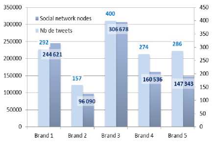
Fig.4. Dataset description

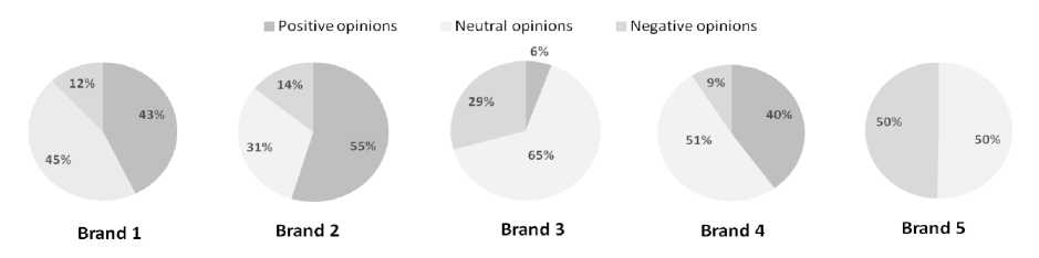
Fig.5. Polarity of opinions in dataset

The first dataset constitutes the initial state and is used to experience the propagation module of IRMS. The second dataset, which contains information of real propagation, is used for comparison and accuracy proof. Before unfolding the reputation measuring process of IRMS, tweets collected are analyzed to extract the opinion they express and the context they belong to. For this purpose, we use existing Python’s API of sentiment analysis and text mining. Once Data set is ready, we measure the reputation score according to the real data collected in the initial state. The group of reach in this case is composed of messages’ authors and their neighbors. Then, we unfold reputation prediction algorithms and estimate the propagated messages. We therefore measure reputation according to forecasted group of reach which is composed of influenced users and their neighbors. Thereafter, we measure the reputation score according to the second dataset which constitutes the real propagation of the initial set. This score is then compared to the reputation measured on the basis of the predicted propagation. In Fig. 6 we represent, for each brand, three reputation values: initial reputation, final reputation and predicted reputation. The graph shows a noticeable variation between the initial and the final reputations regardless of the polarity of the reputation score (positive or negative). This variation is due to the propagation of messages collected in the first dataset, which impacts a larger community in the social network. When we apply our e-reputation prediction model, we obtain a reputation variation very close to the one recorded in the case of real propagated data, and the absolute value of error rate ε between forecasted reputation and final reputation is lower than 1% for all targeted brands. This result shows the accuracy of the prediction model proposed for different brands and with different levels of appreciation in the community.

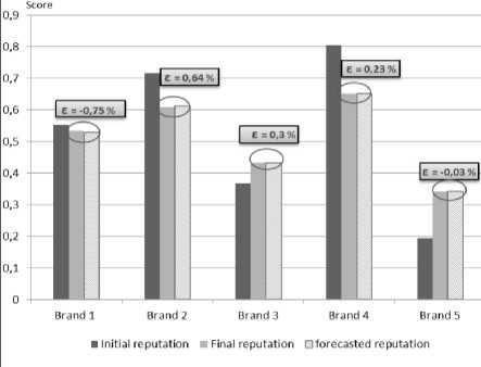
Fig.6. Comparing Forecasted and real final reputation

• VI. C onclusion

In previous works, we presented our Intelligent Reputation Measuring System (IRMS) which measures reputation in social networks using a Bayesian model. In this paper, we focus on a reputation prediction added module which estimates reputation evolution based on propagation algorithms. After describing IRMS model and processing the steps, we give an overview of influence propagation models then we present our proposed prediction algorithms whose accuracy is experimented using real data collected from Twitter. Results reveal an error rate less than 1% between the expected reputation and its real score. However, some challenges remain. Messages collected by IRMS from social network are supposed authentic. But in reality, results can be biased by generating fake messages in the network. IRMS should be able to insure authenticity of messages collected before processing it. IRMS model for measuring reputation can also be enhanced by collecting messages across different social networks and constituting a combined group of reach. These issues are interesting to address in future work.