Ear Biometric System using GLCM Algorithm

Published Online October 2017 in MECS

Biometric Authentication is any process that validates the identity of a user who wishes to sign into a system by measuring some intrinsic characteristic of that user. The need for this technique is further amplified by public safety and national security agencies for whom this is the most secure and accurate authentication tool. Ear images can be acquired in a manner similar to face images.

Figure 1 shows the structure of an ear. Lobule or earlobe is the outer part of the ear. Shadows caused by helix, tragus and antitragus are often seen disrupting the analysis of ear in testing images but these can be removed once the enhancement of image is performed to bring out the useful information from the ear. Many research studies have proposed the ear as a biometric. The human ear has many advantages over other parts of the body used in biometric systems. Researchers have suggested that the shape and appearance of the human ear is unique to each individual and relatively unchanging for a considerable long period of time, unlike the fingerprints which begins to fade away very soon after sixty years of age. It is known that the human ear tends to change its shape and size till seven years of age and remains relatively the same until the person turns eighty. After eighty, the stretch rate due to gravity is not linear, but it mainly affects the lobe of the ear. So the stability and predictable changes makes the ear biometric system more reliable and trustworthy for the organisations where personal security is of utmost importance.

EXTERNAL EAR

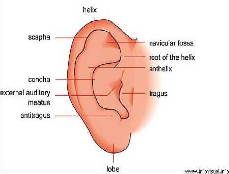
Fig.1. Structure of an Ear

This paper focusses on the GLCM algorithm used to detect the ear properties out of a given data set that is more canonical and precise which paves away the possibility of getting any error. Here we present a step-by-step procedure extending our discussion to seven different steps starting from loading our datasets into database and processing them to final recognition of an ear followed by exit of the whole system.

This paper is organised as follows: A review of related work is given in Section II. Section III describes about the algorithm used in this system followed by Section IV where the whole system is described in a linear and guided fashion. In Section V we present the implementation of this system into real world through an example. This is followed by conclusion and then references.

• II.    Related Work

Due to number of advantages over the face such as no aging and expression problem for adults, smaller size so as to allow less storage requirement and lower computational cost, uniform distribution of colour, etc. the ear has received increased attention as a means to identify people in constrained and unconstrained applications. It is proved medically that the structure of an ear changes during the period from four months to eight years and then gets reformed after seventy years due to aging. Hence ear features are promising biometric for use in human identification because of its stability, uniqueness and predictable changes [1], [4], [5], [6], [15].

Iannarelli is best known as a person who first used ear for identification using a manual technique. His technique was anthropometric in nature, meaning the proportions and measurements of human ear were examined thoroughly by Iannarelli using some ten thousand ear samples. The results of this work indicates that by using limited number of characteristics and features, ear may be uniquely distinguishable and could be used for identification.

Moreno et al. experimented with 2D intensity images of the ear from a collection of 48 people, 28 being in the gallery and the rest apart from the gallery. Three methods were considered for this experiment namely, Borda, Bayesian and Weighted Bayesian. Moreno et al. found the success rate to be 93 percent for the best among three approaches.

Principal Component Analysis or PCA method for ear biometrics on 2D intensity images has been explored by Victor and Chang [6]. PCA method can be used for either facial recognition or ear recognition. Victor and Chang compared their studies on ear authentication with the performance of facial biometrics. Chang’s study saw the similarity in performance of both ear and faces recognition, while the performance of Victor’s study on ear biometrics was worse than that of face. Chang advocated that the difference might be due to differing ear image quality in the two studies.

Another experiment on ear recognition was performed by Choras whose research was based on geometric feature extraction. According to their claims and findings, an error-free recognition can only be acquired on “easy” images or the images which have considerably improved quality.

The two people whose name always comes up when discussing about ear recognition method are Bhanu and Chen. They used local surface shape descriptor [4] as their means to detect ear. In [2], Chen and Bhanu use Iterative Closest Point or ICP algorithm on a sample of thirty 3D ear images. They reported 2 incorrect matches out of 30 persons.

A significant contribution in the field of ear recognition of 2D image was made by Hurley et al. This experiment was based on a technique known as force field transformation. Here a total of 252 images were collected from 63 distinct subjects, getting four images of a single subject. A success rate of 99.2 percent was recorded for this experiment on a given data set. A major drawback that Hurley et al. faced was the failure of this technique for images that were not a part of the data set. The data set images for this experiment must be a collection of ears excluding the ones which have piercings in them or the ones where a significant part of the ear is encrusted by hair.

The researchers happen to find out that the texture plays an important role in the interpretation of digital images. Image segmentation and classification, biomedical image analysis, automatic detection of surface defects are some of its applications worth noticing. The different texture configurations provide us delicate information about the surface of an ear. The textural features with grey-tone spatial dependencies constitute a good application in image classification. Haralick et al. was the first person to use GLCM algorithm. Basically, Grey Level Co-occurrence Matrix or GLCM is an algorithm defined by a two dimensional histogram of grey levels for a pair of pixels, which are separated by a fixed spatial relationship. It is a widely used texture descriptor with proven results about the advantages cooccurrence matrices bear which are not to be seen in other texture discrimination methods. In GLCM algorithm, various co-occurring pairs of pixels are related with reference to the angular and distance spatial relationships when two pixels are considered together at a time.

• III.    Glcm Algorithm

Grey Level Co-occurrence Matrix (GLCM) is an algorithm to determine the texture of an image, be it a face or an ear image. It uses the grey level intensities to obtain a matrix for each and every image. These features of GLCM algorithm are useful in image and texture recognition [3], image retrieval [8], classification of images [9] [10], etc. Taking into account a number of applications possessed by this method, present work deals with analysis of human ear using GLCM algorithm implemented in MATLAB language.

• A.    Texture features extraction from GLCM

Texture feature analysis of second order uses the cooccurrence matrix developed from grey scale images of the human ear.

• B.    Grey Level Co-occurrence Matrices (GLCM)

According to [11], the Grey Level Co-occurrence Matrix algorithm is used for texture analysis in images, especially analysing stochastic textures. Basically it is the tabulation to determine various combinations of pixel brightness values in a given image. Hence it can be defined as a two dimensional histogram of grey levels for pair of pixels, which are separated by fixed spatial relationship.

GLCM of an image is computed using a displacement vector d , defined by radius sigma and orientation theta [12]. Let us take an example of a 4x4 image represented by Table 1 with grey tone values as 0,1,2,3. A generalised GLCM for a particular image is shown in Table 2. Here #(i,j) is a function which produces only those outputs where the grey tones i and j satisfy condition given by displacement vector d.

Correlation is a feature by which the relation between a reference pixel and its neighbour is determined. Mean and standard deviation of both row and column are used to find out the equation of correlation. Mathematically, it is formulated as:

m " { i X j } x ( ^GLCM ( i , j )) - { ^ x X Ц у }

Correlation: XX--------------------------- (4)

Table 1. Test Image

0	0	1	1
0	0	1	1
0	2	2	2
2	2	3	3

Table 2. General Form of GLCM

Grey tone	0	1	2	3
0	#(0,0)	#(0,1)	#(0,2)	#(0,3)
1	#(1,0)	#(1,1)	#(1,2)	#(1,3)
2	#(2,0)	#(2,1)	#(2,2)	#(2,3)
3	#(3,0)	#(3,1)	#(3,2)	#(3,3)

C. Feature Extraction

Feature extraction in GLCM works by picking out various features with the help of next neighbouring pixel in an image, for example, GLCM ( ) is the twodimensional function which takes i, j as inputs. Here i and j are horizontal and vertical coordinates of an image with m pixels in vertical direction and n pixels in horizontal direction. First the intensity contrast between two neighbouring pixels is determined for an entire image. It is calculated as:

Contrast: X X ( г - j )² GLCM ( г , j )        (1)

i = 1 j = 1

Next is the Energy from obtained. This tells us that will be formed due to the level distribution.

which textural uniformity is maximum energy of texture periodic uniformity in grey

mn

Energy: ££ ( GLCM ( i , j ))²         (2)

i = 1 j = 1

Then the Homogeneity which is, the closeness of grey levels in the spatial distribution over image, is recognised. There is a limited range of grey levels in the homogenous textured image so there are very few values having high probability.

• IV. Ear Recognition

This is the section where the algorithm will be actually used to recognise and authenticate the user’s ear and throw an error whenever an intruder tries to enter the private area in a real life scenario. There are six subparts in this section which will guide through every step clearly on how we can use GLCM algorithm to authenticate an ear and use it as a biometric system in day-to-day life.

• A. Loading the Datasets

Here the different structures of human ear will be taken as the dataset. Any human ear, be it of any structure, cannot be taken as it is for recognition without any preprocessing techniques such as conversion of colour image to grey scale. The effectiveness of the system will be maximum only when specific properties has been taken out from the image of an ear that maybe useful for authentication. The main design of the system is that there will be a database which will store certain number of images of the ear that are legitimate. Using the GLCM algorithm, a matrix will be saved for each and every image. Now any one ear will be taken as the test input and will be fed into the system. Corresponding matrix will be generated after a series of pre-processing steps that will then be matched with one of the matrices already stored in the database. If there is a match, the equivalent user will be authenticated and will be declared legitimate; else the user is declared as fraud and will not be granted access. The dataset chosen for this system are given below.

Here Fig. 2a, 2b and 2c shows all the legitimate user ears for whom the authentication will be done and Fig. 3a and 3b shows all the ears not stored in the database, i.e., these ears are not permitted by the system and hence are categorised as fraud. As stated earlier, corresponding matrices will be stored for these ears using the steps described in the following sections.

Homogeneity:

mn

XX i=1 j=1

( GLCM ( i , j )) ¹ + V - ^j\

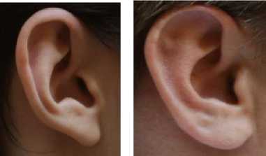
Fig.2a. Legitimate Ears

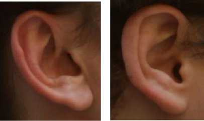
Fig.2b. Legitimate Ears

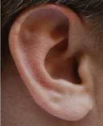
Fig.4. Test Input

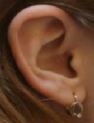
Fig.2c. Legitimate Ear

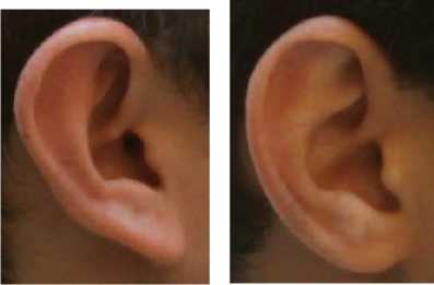
Fig.3a. Unauthorised Ears

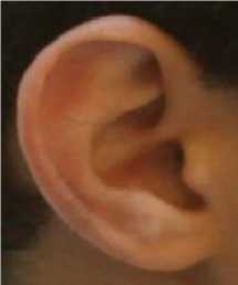
Fig.3b. Unauthorised Ear

• B.    Choosing the Test Case

The next step is to choose the test input for the system. Now for the real life application, this may be done using the CCTV camera in front of any office or institution, but for the sake of implementing the algorithm we’ll select any one of the given test cases from the dataset. The test ear we’ve chosen is shown in Fig. 4.

• C.    Pre-Processing the Test Case

0.2989 * R + 0.5870 * G + 0.1140 * B       (5)

Pre-processing the test input involves conversion of colour image to grey scale image. This is known as rgb2gray conversion. It uses the weighted values of red (R), green (G), and blue (B) components to convert RGB into greyscale image. The process is done as follows:

The next step after rgb2gray scale conversion is finding the histogram equivalence of the given image. A histogram is a graphical representation, usually a bar graph, showing how the numerical data is distributed along the axis. It can also be drawn by calculating the probability distribution of a continuous variable. The following steps are performed to obtain the histogram equalisation of an image:

Step1: First find the number of pixels of image

Step2: Find frequency of each pixel value

Step3: Find the probability of each frequency by dividing the frequency of the pixel with the number of pixels.

Step4: Find the cumulative histogram of each pixel. For the first pixel, it is same as the frequency of that pixel. For the rest, the cumulative histogram is determined by adding the value of cumulative histogram of previous pixel and frequency of current pixel.

Step5: After getting cumulative histogram, find the cumulative distribution probability (cdf) of each pixel by dividing the cumulative histogram of each pixel by the total number of pixels.

Step6: The final value is calculated by multiplying cdf with number of bins.

Step7: Replace the original values in the matrix with final values calculated in step 6.

As an example, Fig. 5a shows the original grey scale image before any pre-processing activity and Fig. 5b shows the histogram equalised image of the original image [13].

From [13], the original histogram of the image is shown in Fig. 6a where it is seen that the lines are not distributed evenly across the whole graph whereas in Fig. 6b, there is a balanced distribution of lines which enhances the image for better productivity of the system.

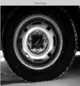
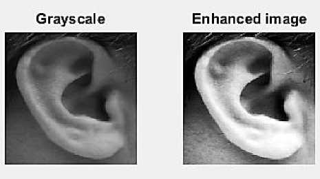
Fig.7. Pre-processed Image of Test Ear

Fig.5a. Original Image

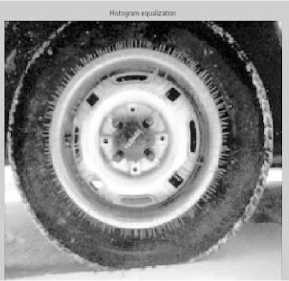
Fig.5b. Histogram Equalisation

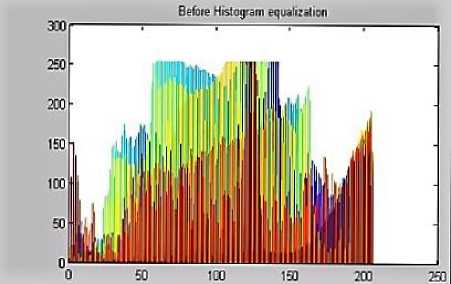
Fig.6a. Original Histogram

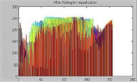
Fig.6b. New Histogram

D. Edge Detection

Edge detection is an image processing technique with the help of which boundaries of objects are gathered in an image. It works by detecting changes and brightness within an image. Besides creating an interesting looking image, edge detection can be a great pre-processing algorithm for image segmentation. For example, if we have a boundary of an object created with edges, it can be filled in to detect the object location. Also if we have two objects that are touching each other or tend to overlap one another, edges can be found and that information could be used to separate the object.

Common edge detection algorithms include Canny, Sobel, Prewitt, Roberts, Laplacian, etc. Prewitt algorithm is used for detecting edges horizontally and vertically. Laplacian operator is also known as derivative operator which recognises second order derivative mask. There are two types of Laplacian operators- positive laplacian and negative laplacian. Sobel operator is well-known operator used for edge detection that can also be categorised as a derivative mask. Sobel operator works be calculating edges in both horizontal and vertical direction. The primary advantage of Sobel operator is its simplicity. But this is accompanied with a disadvantage of being very sensitive to noise. The other kind of edge detection algorithm is Canny operator. It is also known as the optimal detector, developed by John F. Canny in 1986 [14]. It is a multi-step algorithm that detects edges while suppressing the noise at the same time, thus winning over Sobel edge detector algorithm. The steps involved are:

First step is to use a Gaussian filter that has the ability to smooth the image and hence reduce noise, unwanted details and textures.

g ( m, n) = G σ (m, n) * f (m, n)           (6)

Where,

G .

4 2 п. ²

exp(

- m ² + n ²

2 . ²

)

Following histogram equalisation is the process of adjusting the image intensity values in such a way that 1% of data in an image has low and high intensity values. This elevates the contrast of the output image as depicted by the Fig. 7 titled “Enhanced Image”.

Secondly, gradient of g(m, n) is computed similar to Sobel operator.

M (m, n) = 49 m (m,n) + g^ (m,n)     (7)

And

θ (m, n) = tan^-1 [g n (m, n) / g m (m, n)]        (8)

Next, non-maximum suppression is applied in which the algorithm removes pixels that are not part of an edge. If each M T (m, n) term is greater than its two neighbours, then M T (m, n) is kept unchanged, else it is set to zero.

In the final step, thresholding of hysteresis along the edges is done. There are two thresholds used by hysteresis-upper and lower. As in [14], a pixel is recognised as an edge if its gradient is more than the upper threshold and it is discarded if the gradient is less than the lower threshold. If there exists a case where the gradient is in between both the thresholds, then the pixel above upper threshold is recognised as an edge.

Canny operator has many merits than other edge detector algorithms which makes it the most widely used edge detection technique today. Some of them include the smoothening effect for removal of noise, enhancement of signal to noise ratio, effective localization and response, etc. Its weaknesses include the difficulty in implementing the algorithm, time consuming, etc. Given the tremendous and vast advantages this method incorporates, we have used canny operator for edge detection of the ear.

Following image of Fig. 8 represents the output of canny edge detection algorithm for our test case ear as input to the system.

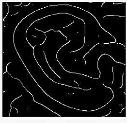
Fig.8. Edge Detection of Test Ear

• E.    Contour Tracing

Contour is an outline representing or bounding the shape or form of something. Contour Tracing is the method of obtaining the outer edge of an ear that has the maximum area of pixels for better identification by the system. This is the last step in processing of ear after which the recognition will take place and the authentication of ear will be determined. For tracking the contour, first step is to label the connected components of an image which is done as follows. In the beginning, a structuring element B is defined. A matrix known as the label matrix is initialised with zeros. Then a different matrix X with all zero elements is initialised and the digit 1 is placed in the non-zero element position in the input matrix (A) of the given input image after edge detection. Dilation is performed after which an intersection is taken of the output received from last operation with the matrix A. If the matrix Y is not equal to matrix X, last two steps is performed iteratively till we get both the matrices equal. A number N is placed in the same positons in matrix Label, as there are positions in Y such that all non-zero elements occupy those positions. Similarly, all zeros are placed in those positions in the input matrix A. This iteration continues till there is a position for every nonzero element in matrix A. Finally the output will be a matrix having labels for all connected components of an image.

The second step in contour tracing is to measure properties of image regions in Label matrix L. There are different regions for each positive integer element of L. For example, value 1 is assigned to elements that correspond to region 1, value 2 is assigned to elements which belong to region 2 and so on. Every region in the image has a set of properties that can be measured for evaluation. Some of the properties include calculating the area, centroid, bounding box, roundness, perimeter, equiv-diameter, etc. In our case, we’ll calculate the area of the different regions of the test image. To calculate area, the total number of ‘ON’ pixels in the image is required, i.e., the pixels whose magnitude is 1 in the label matrix. This scalar value will be stored in a temporary variable and then next step will be to convert this scalar value to vector using the pre-defined function Area in MATLAB where both value and index term will be stored. In order to obtain the desired contour of an ear, maximum area in every region has to be determined. Using this maximum area and the result obtained from edge detection technique, another process can be applied known as area opening . Area opening is a technique that sheds all the irrelevant components which contains pixels less than maximum number of pixels calculated from a binary image. The basic steps involved in calculation of area opening are as follows. First all the connected components are determined. Then the area for those components is calculated. Finally the area which is lesser than the maximum calculated area is destroyed and the rest is taken. This new value is stored in a new variable and is used for calculation of final output matrix. With the new area matrix as an input to the next function, a grey-level co-occurrence matrix (GLCM) is created using the algorithm described in Section III that will act as the final output of the whole ear detection system after which the recognition part will occur.

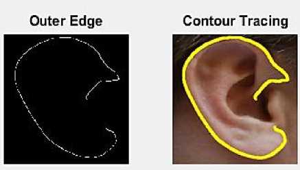
Fig.9. Tracing Contour of Test Ear

In Fig. 9, we can notice how the outer edge of our test case ear is determined accurately that will be used for recognition later. It should be put into utmost notice how the edges from Fig. 8 are eradicated, leaving only the useful and applicable ones in Fig. 9 for ear authentication.

• F.    Ear Recognition

This is the last process of the whole ear detection technique. Here the output matrix from previous step is taken and matched with all the grey-level co-occurrence matrices present in the database that were formed from sample ear images using all pre-processing techniques discussed so far. Once there is a hit, the system will print the “Welcome” message and will do the necessary operations in real time application. If the ear fails to match, the system prints “Unauthorised Access” and denies all the operations for that particular user.

• V.    Implementation of System

In the last section we discussed the various stages of ear detection and authentication system and ended our topic by concluding that when the grey-level cooccurrence matrix of test input matches with that in database, then the system authorises access to the user, otherwise no access is granted. In this section we will talk about how the system will behave in a real-life scenario. Given that the system for recognition is made and now it needs to be implemented on a hardware module, this can be achieved by using an Arduino UNO R3 and a couple of other devices like a transformer, voltage regulator, bridge rectifier, capacitor, buzzer, LCD display, etc. Arduino UNO R3 is an electronic board that is able to read input from the system and turn it into a desired output. Input from the system can be anything, for example, a light on sensor, finger on a button or even a Twitter message. Output produced from Arduino board can range from activating a motor to turning the light of sensor ‘ON’. The Arduino board used in our experiment is shown in Fig. 10.

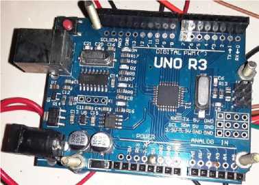
Fig.10. Arduino UNO R3 board

Transformer is an apparatus used for alleviating or increasing the voltage of an alternating current. It does so with the help of a mutual induction between two windings. Now the Arduino board requires 5V power rating in order to operate. One transformer should be enough to supply this much amount of voltage to the electronic board but not enough to operate all devices properly. Hence two transformers are attached with

Arduino board to regulate sufficient power among all connected devices for improved performance. LCD screen display is attached with the board to monitor every detail visually and see the corresponding output. The screen will display “Authorisation Success” for the individuals whose ear get authenticated and will pop up “Unauthorised Access” for all users who are not authenticated with database. Similarly a buzzer is attached with board which will go off as soon as there is an incorrect match, thus alerting the staff members of the intrusion. Apart from this, a GSM module is also tethered to the Arduino for added security. Through GSM module, a specified mobile number would get notified whenever there is person entering the private area or if someone tries to break-in when the system does not authenticate the intruder. This way the user will not be given access to certain restricted areas and the owner of the place will be intimidated via messages of the events happening in their absence. The following figures exhibits some of these electronic devices.

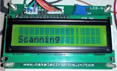
Fig.11. LCD Display

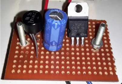
Fig.12. Voltage Regulator, Capacitor, Rectifier

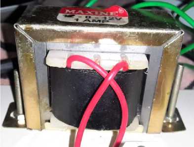
Fig.13. Transformer

These devices can be arranged in a systematic manner to form a complete unit that would trigger an alarm when there’s no ear match for a particular user while displaying corresponding message on LCD screen. If there is a perfect match, a motor could be made to spin that would further produce some desired output. The complete arrangement of devices is shown in Fig. 14.

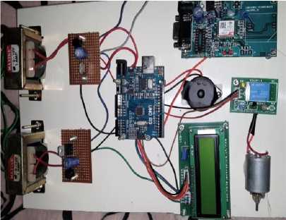
Fig.14. Complete Circuit

• VI.    Conclusion

This paper presented an efficient and an orderly way of ear biometric system using GLCM algorithm. Having mentioning briefly about the advantages a human ear has over other biometric parts, this work described how an ear biometric system can be constructed using steps that convert a test ear into GLCM matrix in order to accurately authenticate it. Next the implementation of this system was presented that exhibited how using some electronic components along with Arduino board, the method will function thus giving an idea of its unambiguity in real-life scenarios.