Efficient and Fast Initialization Algorithm for K-means Clustering

Published Online February 2012 in MECS

• A.    Motivation

Large amount of data is being collected every day in many business and science areas [1]. This data needs to be analyzed in order to find interesting information from it, and one of the most important analyzing methods is data clustering.

Clustering is one of the most important data mining tools which help data analyzers to understand the natural grouping of attributes in the data [2]. Cluster analysis is used in many field such as data mining [3], pattern recognition and pattern classification [4], data compression [5], machine learning [6], image analysis [7], and bioinformatics [8].

Data clustering is a method in which a cluster of objects is made that are somehow similar in characteristics. The criterion for checking the similarity is implementation dependent.

Figure 1-a shows many points plotted in 2D space, these points may share some kind of similarity between them. Data clustering is to group similar data together to form a cluster as shown in Figure 1.b.

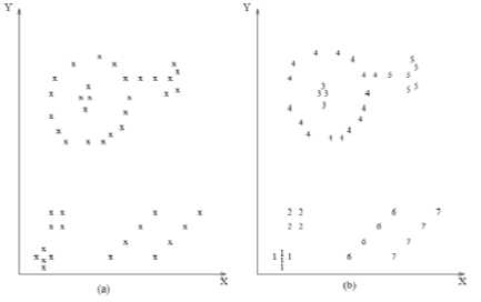
Figure 1: Data Clustering

Existing clustering algorithms can be classified into two major classes, hierarchal and partitioning algorithms. A hierarchal method uses a nested sequence of partitions. This can be done by considering all data as one cluster and then dividing it into smaller ones, this is called Divisive clustering. The other class consider each data point as cluster and then merges them to form bigger cluster, this is called Agglomerative clustering [9].

• B.    Components of a clustering task

Typical pattern clustering activity involves the following steps [10]:

• •    Pattern representation.

• •    Definition of a pattern proximity measure appropriate to the data domain.

• •    Clustering or grouping

• •    Data abstraction (if needed)

• •    Assessment of output (if needed).

• C.    Similarity measure

Since similarity is fundamental to the definition of a cluster, a measure of the similarity between two patterns drawn from the same feature space is essential to most clustering procedures. Because of the variety of feature types and scales, the distance measure (or measures) must be chosen carefully. It is most common to calculate the dissimilarity between two patterns using a distance measure defined on the feature space. There is a lot of similarity measures like Manhattan Distance, Maximum Distance, Minkowski Distance and Mahalanobis Distance [11]. The most popular metric for continuous features is the Euclidean distance.

Euclidean distance or Euclidean metric is the "ordinary" distance between two points that one can measure with a ruler, and is given by the Pythagorean formula (Eq.1).

The Euclidean distance has an intuitive appeal as it is commonly used to evaluate the proximity of objects in two or three-dimensional space. It works well when a data set has “compact” or “isolated” clusters [12].

• D.    Partition Clustering Algorithms

A partition clustering algorithm obtains a single partition of the data instead of a clustering structure, such as the dendrogram produced by a hierarchical technique. Partition methods have advantages in applications involving large data sets for which the construction of a dendrogram is computationally prohibitive. A problem accompanying the use of a partition algorithm is the choice of the number of desired output clusters.

One of the most famous partition algorithms is the K-means. The K-means is the simplest and most commonly used algorithm employing a squared error criterion [13]. It starts with random initial centroids and keeps reassigning the patterns to clusters based on the similarity between the pattern and the cluster centroids until a convergence criterion is met after some number of iterations. The K-means algorithm is popular because it is easy to implement, and its time complexity is O (n), where n is the number of patterns. The basic algorithm works as follows:

Algorithm 1 : Basic K-means

• 1-    Select random K points as initial Centroids

• 2-    Repeat

• 3-    Form K clusters by assigning all points to the closest centroids

• 4-    Recompute centroids for each cluster

• 5‐    Until The Centroids don’t change

Note that K-means [14] is defined over numeric (continuous-valued) data since it requires the ability to compute the mean. A discrete version of K-Means exists and is sometimes referred to as harsh EM [15].

The rest of this paper is organized as follows: section 2 introduces some of the related works and some previous solutions to the K-means initialization problems. Section 3 introduced the proposed algorithm and our new framework. Section 4 provides the simulation results and section 5 gives the conclusions.

• II.    RELATED WORK

The K-means algorithm finds locally optimal solutions minimizing the sum of the L2 distance squared between each data point and its nearest cluster center [16,17], which is equivalent to maximizing the likelihood given the assumptions listed above.

A major problem with this algorithm is that it is sensitive to the selection of the initial partition and may converge to a local minimum of the criterion function value if the initial centroids are not properly chosen.

There are various approaches to solving the problem of determining (locally) optimal values of the parameters given the data Iterative refinement approaches, which include EM and K-means, are the most effective.

Several methods are proposed to solve the cluster initialization for K-means. A recursive method for initializing the means by running K clustering problems is discussed in [14]. A variant of this method consists of taking the entire data and then randomly perturbing it K times [18]. Bradley and Fayyad in [19] proposed an algorithm that refines initial points by analyzing the distribution of the data and probability of the data density. In [20] they presented empirical comparison for four initialization methods for K-means algorithm and concluded that the random and Kaufman initialization method outperformed the other two methods with respect to the effectiveness and the robustness of K-means algorithm. In [18] they proposed Cluster Center Initialization Algorithm (CCIA) to solve cluster initialization problem. CCIA is based on two observations, where some patterns are very similar to each other. It initiates with calculating the mean and the standard deviation for data attributes, and then separates the data with normal curve into certain partition. CCIA uses K-means and densitybased multi scale data condensation to observe the similarity of data patterns before finding out the final initial clusters. The experiment results of CCIA performed the effectiveness and robustness of this method to solve the several clustering problems [21].

In [22] Al-Daoud introduced a new algorithm for initialization. The idea of the algorithm is to find the dimension with maximum variance, sorting it, dividing it into a set of groups of data points then finding the median for each group, using the corresponding data points (vectors) to initialize the K-means. The method works as follows:

• 1.    For a data set with dimensionality, d, compute the variance of data in each dimension (column).

• 2.    Find the column with maximum variance; call it cvmax and sort it in any order.

• 3.    Divide the data points of cvmax into K subsets, where K is the desired number of clusters.

• 4.    Find the median of each subset.

• 5.    Use the corresponding data points (vectors) for each median to initialize the cluster centers.

The use of median in this method makes the algorithm sensitive to outliers.

• III.    Proposed Work

• A.    Overview

  A visual clustering framework is build using C++ Builder 2009.This frame work allows us to generate datasets using a graphical user interface (Figure 2) and allows us to load datasets from different sources and

represent it using 2-D graphics. It also allows us to implement different clustering algorithms and test them. In our case the k-means algorithm and the new initialization algorithm ( ElAgha initialization ) are implemented.

This framework (Figure 3) allows us to select the initialization for the points from three methods. 1-Random initialization. 2- Manual initialization. 3-ElAgha initialization. Random initialization selects randomly K centroids points, Manual initialization allow the user to select K points manually and place them using the mouse any where he wants and ElAgha initialization select K points using the proposed algorithm.

The statistics widow shows us how many iterations used to finish clustering and shows us the overall error value.

ElAgha initialization generates K points using semi random technique. It makes the diagonal of the data as a starting line and selects the points randomly around it.

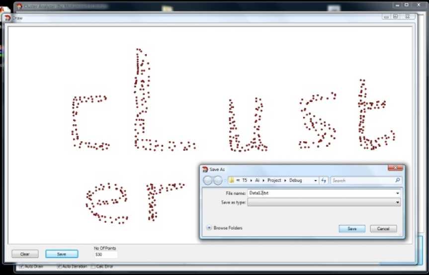
Figure 2: Draw Form

Figure 2 shows easily how any artificial data sets are generated by just drawing it using the computer mouse. After this it can be saved as a text data file that can be easily loaded using any clustering framework.

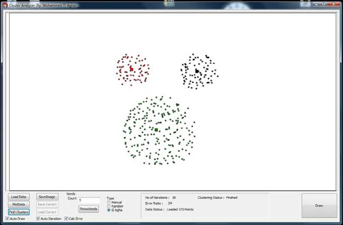
Figure 3: Main Framework Form

Figure 3 shows how the main framework form loaded the Mickey Mouse dataset and clustered it using ElAgha initialization with three points. It also shows how many iterations it uses to finish the clustering and the error rate duo to it.

• B.    ElAgha initialization.

ElAgha initialization is a new algorithm that generates initial K-means centroids depending on the overall shape of data. Note that the algorithm will explained using 2D space in order to make it easy to understand, but it can easily work on higher dimensions as we will see next when real datasets are tested.

ElAgha initialization first finds the boundaries of data points, and then it divides the area covered by the points into k rows and k columns forming a 2D grid. The width of the grid cell ( Xw ) is calculated using Eq.2:

Xmax — Xmtn

К

Where Xmax = the biggest X value from all points and Xmin is the smallest one.

The height of the grid cell ( Yw ) is calculated using Eq.3 :

Ymax — Ymin

K

Where Ymax = the biggest Y value from all points and Ymin is the smallest one.

ElAgha initialization then uses the upper left corner of the cells lied on the diagonal as a base points that will be used to generate the actual initial centroids. Initial centroids are a random bias from base points that can move left for up to Xw/2 in X-axis and up to Yw/2 in Y-axis. And can moves right up to Xw in X-axis and up to Yw in Y-axis. Figure 3 shows the possible locations of the initial centroids for the Mickey Mouse dataset using ElAgha initialization.

The semi random technique is used in order to make each initialization different from the other for the same dataset, and that is to make a chance for the algorithm to success in next run of the code if it failed from the previous run.

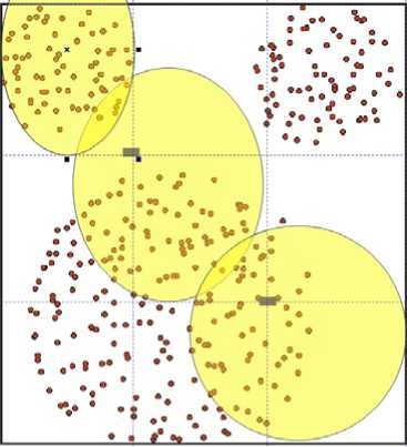
Figure 4: Possible locations of initial centroids for the Mickey Mouse dataset using ElAgha initialization.

Algorithm 2 shows ( ElAgha initializations) actuall work implemented using C++, note that (Xc ,Yc) is the initial starting point and CandidatesCents array is a 2D array that candidate initial centroids where stored in it. For our assumption the diagonal of the array is used as our initial points.

Algorithm 2 : ElAgha Initialization

• 1-    Get Points Covered area Xc=Xmin ,Yc=Ymin

• 2-    Compute Xw=Area width/K

• 3-    Compute Yw=Area height/K

• 4-    for (int n =0 ;n < K; n++) {

• 5-    for (int i = 0; i < K; i++)            CandidatesCents[i][n].X=

Xc+random(Xw)-random(Xw/2);

• 6-    CandidatesCents[i][n].Y=

Yc+random(Yw)-random(Yw/2);

• 7-    Xc+=Xw ; }

• 8-    Xc=xMin;

• 9-    Yc+=Yw; }

• 10 ‐ Centrodes is the diagonal points in the CandidatesCents Array

• IV.    SIMULATION & RESULTS

• A.    Experimental Methodology

The problem of initializing a general clustering algorithm is addressed , but limit the presentation of results to K-means. Since no good method for initialization exists [23], a comparison against the standard method for initialization is made: randomly choosing an initial starting points.

ELAgha initialization and the traditional random initialization algorithms is executed for 10 times in order to compare between them. Our algorithm is tested using artificial and real datasets.

• B.    Artificial Datasets Results

Artificial datasets are built using our new framework. Three different datasets are built. Dataset-1 Consist of 320 points and 8 clusters (Figures 4). Dataset-2 Consist of 373 points and 3 clusters (Figures 5). Dataset-3 Consist of 211 points and 6 clusters (Figures 6).

The following measurement factors are used in order to compare:

• a.    Average SSE.

• b.    Miss classified samples (average error index).

• c.    Average no of iterations to find correct cluster

Table 1 summarizes error ratio test for the data. The traditional and ELAgha initializations are executed for 10 times and the average SSE is calculated using Equation 4:

£i=l ErrorCi) Average SSE = ----—----    (4)

Where Error (i) is the within-cluster sum of squares (WCSS) value of the ith run, S is the space of the K cluster and calculated using Equation 5:

к

55E = ^^VXj - ц(^2  ( 5)

i=l xjes

As shown in (Table 1) ELAgha initialization outperformed the traditional random initialization by a big factor especially in complex datasets. For example Random Initialization get average error for Dataset-1 equal to (168270) and ELAgha initialization gets (125801), so it performed better with a factor of (1.3). For the complex Dataset-2 ELAgha initialization performed better with a factor of (3.74).

Table 2 summarizes the average error index for both algorithms in 10 runs which are calculated using Equation 6. For Dataset-1 Traditional initialization got an average error index of 65% but ELAgha initialization got only 2.27%.

Count of misclassified samples

Error Index = ---------------—p— x 100% 6)

Total No of samples

Table 3 shows that for Dataset-2, Traditional initialization got an average error index of 43.4%. In the other side ELAgha initialization got only 5%.

Table 4 shows that for Dataset-3 , Traditional initialization got an average error index of 56.47 % and ELAgha initialization got 4.44 %.

Table 5 illustrates the average no of iterations both algorithms needed to finish successfully clustering. For Dataset-1 Traditional initialization needs an average of 23 iterations to find correct clusters and ELAgha initialization needs only an average of 14 iterations. For Dataset-2, Traditional initialization didn’t success at all to find correct clusters and ELAgha initialization needs an average of 33 iterations to find them. Finally for Datase-3, Traditional initialization also didn’t success at all to find correct clusters and ELAgha initialization needed an average of 36 iterations.

TABLE 1: AVERAGE ERROR FOR 10 ITERATIONS FOR 3 DATASETS

	Dataset 1	Dataset 2	Dataset 3
Average error for 10 iterations for the traditional initialization	168270.1	193049.7	105125.9
Average error for 10 iterations for ElAgha initialization	125801.8	51569.3	93329.5

TABLE 2: AVERAGE ERROR INDEX FOR DATASET 1

	1	2	3	4	5	6	7	8	9	10	Average
Traditional initialization	50	25	50	25	25	75	50	25	12.5	0	65
ElAgha initialization	10.9	0	11.8	0	0	0	0	0	0	0	2.27

TABLE 3: AVERAGE ERROR INDEX FOR DATASET 2

	1	2	3	4	5	6	7	8	9	10	Average
Traditional initialization	74.7	80.4	50.1	77.7	2.68	50.1	13.4	5.36	26.8	53.6	43.4
ElAgha initialization	0.26	49.8	0	0	0	0	0	0	0.52	0	5

TABLE 4: AVERAGE ERROR INDEX FOR DATASET 3

	1	2	3	4	5	6	7	8	9	10	Average
Traditional initialization	18.9	21.3	71	37.4	52.6	68.2	66.3	36.9	69.6	56.3	56.47
ElAgha initialization	0	23.6	0	0	0	0	0	0	0	20.8	4.44

TABLE 5: AVERAGE NO OF ITERATION TO FINISH CLUSTERING FOR CORRECT CLUSTERS OF THE K-MEANS

	Dataset 1	Dataset 2	Dataset 3
Traditional initialization	23	Never Succeeded	Never Succeeded
ElAgha initialization	14	33	36

• C.    Real Datasets Results

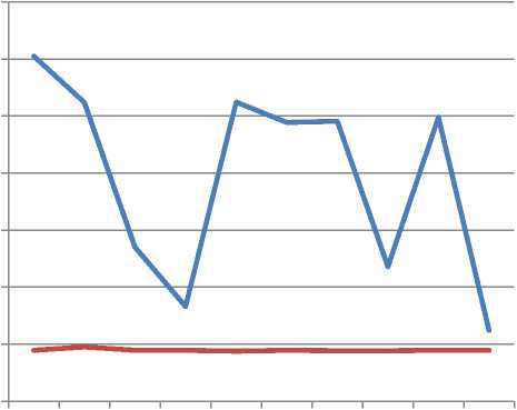
For real data, the iris data set from the UCI is used which contains three clusters, 150 data points with 4 dimensions data. For Error validation and comparison between our algorithm and the traditional algorithm, Average Error value and the error index which are calculated from equations 4, 6 respectively are used. Table 6 first row shows the error value duo to the use of traditional initialization method for each one of the 10 runs. Row 2 shows the error duo to the use of ElAgha initialization. Row 3 shows the improvement in reducing the error rate when using ElAgha initialization and this value is calculated using Equation 7.

Improvment =

Error duo to traditional initialization

Error duo to ElAgha initialization

Table 6 shows that for real datasets, ElAgha initialization produced a stable and better error value than traditional initialization. The average error value for ElAgha initialization was (44802.8) and for the traditional initialization was (196328) which is more than 4 times average improvement.

For error index validation, ElAgha initialization gets 11.3% missed classifications and traditional initialization got 48% .

Chart 1 shows a graphical plot of Table 6. It clearly shows that ElAgha initialization is a way better than traditional initialization in error value, as it is has stable and a lower error values .

TABLE 6: ERROR COMPARISON BETWEEN TRADITIONAL INITIALIZATION AND ELAGHA INITIALIZATION FOR 10 RUNS OF IRIS DATASET

	1	2	3	4	5	6	7	8	9	10	average
Traditional	302567	261895	134941	82937	262245	244412	245380	117927	248986	61999	196328.9
ElAgha	44688	47516	44647	44688	43916	44688	44274	44274	44649	44688	44802.8
Improvement	6.770654	5.511722	3.022398	1.855912	5.971514	5.469298	5.542305	2.663572	5.576519	1.387375	4.377127

^^^^^^еTraditional

^^^^^^е El Agha

123456789 10

Chart 1: Comparison between the error values when running ElAgha initialization Vs traditional initialization for 10 times run of the algorithm

V CONCLUSIONS

It is widely reported that the K-means algorithm suffers from initial cluster centers. Our main purpose is to optimize the initial centroids for K-means algorithm. Therefore, in this paper ELAgha initialization was introduced. It is an initialization algorithm that uses a guided random technique. Experimental results showed that ELAgha initialization outperformed the traditional random initialization and improved the quality of clustering with a big margin especially in complex datasets.