Efficient classification using average weighted pattern score with attribute rank based feature selection

Автор: S. Sathya Bama, A. Saravanan

Журнал: International Journal of Intelligent Systems and Applications @ijisa

Статья в выпуске: 7 vol.11, 2019 года.

Бесплатный доступ

Classification is found to be an important field of research for many applications such as medical diagnosis, credit risk and fraud analysis, customer segregation, and business modeling. The main intention of classification is to predict the class labels for the unlabeled test samples using a labelled training set accurately. Several classification algorithms exist to classify the test samples based on the trained samples. However, they are not suitable for many real world applications since even a small performance degradation of classification algorithms may lead to substantial loss and crucial implications. In this paper, a simple classification method using the average weighted pattern score with attribute rank based feature selection has been proposed. Feature selection is carried out by computing the attribute score based ranking and the classification is performed using average weighted pattern computation. Experiments have been performed with 40 standard datasets and the results are compared with other classifiers. The outcome of the analysis shows the good performance of the proposed method with higher classification accuracy.

Еще

Classification, outlier detection, pattern matching, feature selection, attribute rank score

Короткий адрес: https://sciup.org/15016607

IDR: 15016607 | DOI: 10.5815/ijisa.2019.07.04

Текст научной статьи Efficient classification using average weighted pattern score with attribute rank based feature selection

Published Online July 2019 in MECS

Due to the technological improvement and growth of emerging technologies, the storage of data in all fields is getting multiplied for every microsecond. This explosive growth of collected data has to be analyzed for extracting valuable information and to transform them into interesting knowledge. Classification and predictions are the two main areas that are focused on almost all the fields for improving the trends, making decisions and predicting future events based on the collected data. Data mining and machine learning algorithms, generally build a mathematical model on the training sample dataset, in order to make forecasts or decisions by analyzing the data. Data mining is the process of discovering patterns in large data sets from various applications involving methods at the intersection of machine learning, statistics, and database systems [1]. Data Mining is the technical base for Machine learning (ML) which is the study of algorithms and mathematical models used to improve the performance of the applications [2].

Supervised learning is the primary context in data mining and machine learning fields. In general, supervised learning creates and trains a model to predict the future based on the results from the analysis of past history. More technically, supervised learning algorithms have a set of training samples each of which has the input object (set of attributes) and output object (class labels). Once the unlabeled test samples are given as input to the supervised learning algorithm, it examines the characteristics and class labels of training samples and based on which it predicts the class labels for the unlabeled input test samples [3]. Thus, categorizing, classifying or predicting the class labels for unlabeled test samples with the help of a trained model is known as classification. Several classification algorithms are generally available in data mining and machine learning context.

In the classification problem, feature selection is an important task which includes selecting the relevant feature for constructing the model as the dataset contains some features that are redundant and irrelevant features. These irrelevant features that are not interesting for the study can be removed during the classification process [4]. Some of the classification algorithms that are used widely in various applications are eager learners such as Artificial neural networks [5], decision trees [6], naïve bayes [7], instance based classifiers [8] such as nearest neighbour [9], statistical models such as linear regression [10], logistic regression [11], nature-inspired techniques such as genetic programming [12] and ensemble based learners [13] such as random forest [14], adaboost [15], and support vector machine [16]. Though several methods exist to classify the dataset, they suffer from several issues. Simple methods generally provide low classification accuracy. Many difficult methods even provide misclassification. Pretentious and complex methods that are having high prediction rate, however, suffer from computational complexity.

This paper presents an instance based classifier algorithm with an average weighted pattern score with attribute rank based feature selection to predict the class labels for the unlabeled test samples. This method is simple however, it produces better classification accuracy than many other traditional methods. An attribute score based ranking algorithm has been proposed to select the relevant attributes by calculating the attribute rank by taking the number of unique values in the set of training samples into account. The attribute rank is converted to attribute weight using the rank sum weight method. The attributes of the test sample are compared with the attributes of the training samples to find the matched pattern. The pattern score of the test sample for each training sample is calculated using the attribute weight and are grouped based on the class label. The average pattern score for each group is calculated and the class group having a maximum score is predicted as the class label for the unlabeled training sample. The experimental study has been performed with 40 standard datasets available at UCI [17] and KEEL [18] repository. The proposed algorithm is compared with other existing methods and the classification accuracy and AUC values are evaluated and analyzed using statistical tests. Through the analysis, the proposed system provides better results than other algorithms.

The organization of the paper is as follows. Section II presents the related work from the literature survey. Section III explains the proposed methodology in details. Experimental analysis is presented in section IV with experimental setup and result analysis. Finally, the paper concludes the work with a conclusion.

II. Related Works

Several methods and their variations exist in the literature for classifying the unlabeled samples. Eager learners generally create a learning model based on the training data and classify the unlabeled sample based on the created model. An artificial neural network is an idea inspired by biological neural networks with a system of interconnected ‘neurons’ calculating values from the input. Even if the implementation of the model is simple, the processing time increases with the increase in the neural network and are prone to overfitting [19]. Decision trees are tree based predictive model that identifies the target class for the given sample by partitioning the trained samples. The main drawback of decision trees is that in some cases the splitting process may lead to loss of information [20]. Another common eager learner is naïve bayes classifier. It is a probabilistic predictive model that applies Bayes theorem for predicting the class label. However, the accuracy of the prediction decreases with the decrease in the number of training samples [21].

Given a set of training sample with attributes having numeric values, Linear regression fits a linear function to a set of input-output pairs. [22]. Generally, the model is limited to the linear relationship between a set of dependent and independent variables. Similar to linear regression, Logistic regression can be employed for the binary/multivariate classification task. However, the model works well only if the number of output variables is minimum [23]. The main idea of ensemble-based learners is to convert weak learners to strong learners by applying several homogeneous or heterogeneous classifier model. Random forest classifier usually builds multiple random trees by selecting a random sample with replacement and by selecting random attributes from the training set for classifying the unlabeled test data using majority votes [24]. However, the computational complexity and time to build the random trees are really high. Boosting is a method that involves combining heterogeneous learning algorithms for improving the performance of the system. Adaptive Boosting (AdaBoost) classifier combines several heterogeneous weak classifiers to make a strong classifier. AdaBoost provides better accuracy in classifying data samples but is prone to overfitting [25].

Support vector machine is a good choice for various classification problems. However, choosing the best kernel suitable for the application is difficult. Also, they are prone to noise and missing values [16-26]. Instance based classifiers are the most widely used classification as it is simple and easy to understand. K-nearest neighbor classifier is the simple classification model where the input consists of k nearest training samples and the class label for the test sample is predicted by a majority vote of its neighbors [27]. A new variation of kNN method based on a two-sided mode, called general nearest neighbor (GNN) rule has been suggested. But the main disadvantage of these methods is that they rigorously deteriorate with noisy data or high dimensionality and the performance becomes very slow [28]. In reference [29], Peng et al. (2009) proposed a new instance based classifier named as Data Gravitation based Classification (DGC) [30,31]. This algorithm basically classifies the test samples by comparing the data gravitation between the different data classes. In reference [32], Cano et al. (2013) extended the DGC by improving the classification accuracy and is called Weighted Data Gravitation based Classification (DGC+) but with the highest complexity.

III. Average Weighted Pattern Score with Attribute Rank Based Feature Selection

The proposed classification method uses average weighted pattern score along with attribute rank for feature selection. The PMC algorithm proposed by the authors Sreeja and Sankar [33] has been taken as a base and further extended by introducing the weights and rank weights for the attributes in the process of feature selection. The overall architecture of the proposed methodology is given in Fig.1.

The proposed method uses the attribute scoring based feature selection with the weighted pattern matching mechanism. Consider the dataset D consisting of n attributes denoted by a1, a2, a3, …, an and m instance denoted by i1, i2, i3, …, im. It is depicted in the following matrix form in (1).

Attributes i1

a 1 x 11 ^x 21

a 2 x 12 ^x 22

a n x 1n ^x 2n

In the above matrix x m1 , x m2 , …, x mn are the values of the n attributes of the m ^th instance. Specifically, each instance belongs to a class C k where k takes the values 1, 2, …, p.

As a pre-processing step, the prominence of the attribute in the classification process is calculated. All the attributes are ranked based on their importance. Let R be the ranker function that assigns a value to each attribute a j thatbelongs to the dataset D based on the relevance score. It then returns the list of attributes well-arranged based on their relevancy and the formula is

R ( ci ^ , ci 2 , ci 3 ,.. ci)) — < ci ^ , ci 2 , ci 3 ■ ■ ■ ci^ >. (2)

i m x m1 x m2

x mn

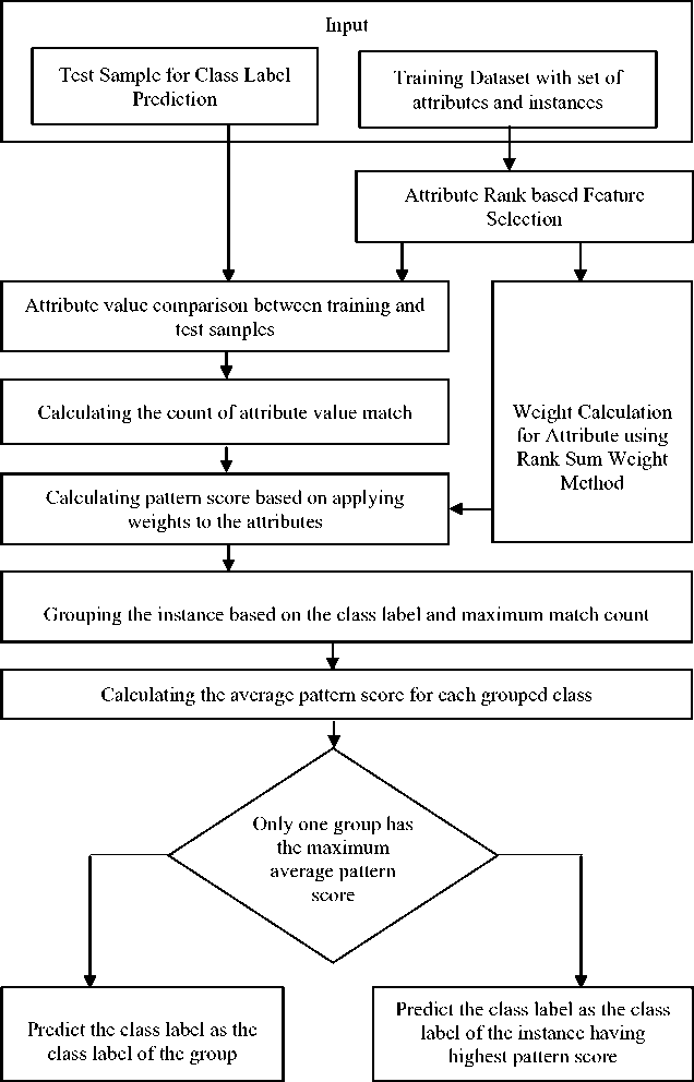
Fig.1. Architecture of the proposed classification method.

Here, the list of attributes a 1^’ , a 2^’ , a 3^’, …, a n^’ take the ranks 1, 2, …, n. The attributes that are not relevant can be removed based on the relevance score. Only the top relevant attributes having the highest score is selected. Let q be the number of attributes selected as relevant for the classification.

Each selected ranked attribute a 1^’ , a 2^’ , a 3^’, …, a q^’ is then assigned a weight based on the rank sum weight method. By using the rank sum weight method, the weights are calculated and are normalized in such a way that the sum of weights of the ranked attributes is 1 and the formula is depicted in (3).

( ( ))

( )=(3)

∑ ( ( ))

The main aim of the proposed classifier is to identify the class label for the unlabeled test instances. The proposed method uses PMC [33] to find the instances with the highest attribute match count by comparing the selected attribute values of the training instances and the test instances as shown in (4) and (5). The matched count of m ^th instance is represented as n_n(m) and the calculation is given in (4).

q na' (m) = ^S(ai) (4)

i = 1

where ( ) is the attribute match score which takes the value either 0 or 1. If the value of attribute ai of the test sample equals the corresponding attribute value of the training sample then the score will be 1 else the score will be 0. This can be represented as in (5).

1, ℎℎ

( )= ℎ ℎ

0,ℎ

The method then selects the training samples having the highest attribute match count with the given test sample. The selected training instances are grouped based on the class labels as shown in (6) [33].

∈ ()= ∈ (6)

c in represents the number of classes in the selected training set samples. All instances having maximum and belonging to the class C j is grouped. The rank weights of the selected attributes are applied to the selected training instances to find the pattern score of the test sample t with respect to the training samples x_i which is represented as PS(x _i ) and the formula is depicted as

PS ( X i) = £ 5 ( a i )* w ( a i ) (7)

i = 1

The average pattern score ( ) of class c is calculated by finding the average score of each group in the selected training set samples. The pattern score of the test sample is the maximum score found among the averaged pattern score of groups . Finally, the class label for the test sample is predicted as the class group having a maximum average pattern score and the details are represented in (8) and (9).

= ( ( )) (8)

^•test ^ Q ( )= (9)

If more than one group arrive the maximum average pattern score, then the class label is predicted using the individual instance pattern score. The class label for the test sample is predicted as the class label of the training instance having maximum pattern score since the topmost attribute that is relevant is highly involved in determining the class label and expression is shown in (10).

(max( ()) (10)

The algorithm pseudocode for the proposed average weighted pattern score with attribute rank based feature selection classifier is presented in Fig.2.

The attribute selection is a significant step that contributes the classification accuracy. It provides a rank for each attribute in the dataset using mathematical measures. Each attribute will be ranked based on the score obtained by them. The attributes having best rank will be considered as the relevant attributes and least scored attributes are considered as the irrelevant attributes which can be removed. The proposed method for attribute score calculation called attribute score based ranking algorithm ASR algorithm is described. Consider the training dataset D with m distinct classes Ci. The overall score of the database based on the number of distinct classes is calculated as in (11).

Score (D) = Avg К>/-)

V i=1

where p i is the probability that an arbitrary instance in D that belongs to class C i . The formula to calculate p i is shown in (12).

Number of instances belonging to Ci

=(12)

Total number of instances in D

To calculate the attribute score for each attribute, having n distinct values, the count of tuples set having n distinct values {n 1 , n 2 , n 3 , …, n j } are grouped as {G 1 , G 2 , …, G j }. The calculation of attribute score A score is given in (13).

^ n ^

AScore = Score ⁽ D ) - Avg ^ P ⁽ nj ) X Score ⁽ Gj ) I ⁽¹³⁾ V 7 = 1 )

where ( ) is the probability that an arbitrary instance in Gj that belongs to class Ci

The score for each attribute is calculated and the rank is evaluated for all the attributes. The attribute score based ranking algorithm is explained in Fig.3.

Algorithm: A WPS Classification

Method : Average Weighted Pattern Score with Attribute Rank based Feature Selection Classifier

Input : Input training set D, unlabeled test sample x test

Output : Predicted class label

Procedure A WPS_ Classifier

Begin m = number of attributes n = number of instances

a[q] = AttributeRank (D)

//q is the number of attributes selected

//calculate the weight of the attribute using rank sum weight method

For j = 1 to q

w[j] = 2*(n-r(j)+1)/(n*(n+1));

End For

For i = 1 to n do

( i )=0;

For j = 1 to q do

If (x test (a[j]) = = x i (a[j])) Then

S(a[j]) = 1;

Else

S(a[j]) = 0;

End If

End For

( i )= ( i ) + S(a[j]);

End For

For i = 1 to n do

Identify the maximum value of the match count

Max( n_a' ⁽ i ) );

End For

Group the instances i based on the class label and maximum match count ik ∈ Gc iff na- (к)=maximum and ik ∈ Cj

For each selected instance i in the group c do

For j = 1 to q do

//Apply weights to the attributes belonging to the each grouped classes and calculate pattern score

PS ( i )= ∑ ⁴i^^S ( a [ i ]) ∗ w( a [ j ]);

//calculate the maximum patter score among the selected instances max( PS ( i )

End For

Calculate the average pattern score for each grouped class

PS ( x_c )

End For

If one group has the maximum average pattern score

Predict the class label as Cj

Xtest e Cj iff PS ( Xc )= max ( PS ( Xc ))

Else Xtest e Class (max( PS ( x ))

End If

End Function

Fig.2. Algorithm pseudocode for the proposed classification method.

To illustrate the attribute score based ranking algorithm, consider the training tuples containing class labels from the AllElectronics Customer Database used by Han et al. (2011) [1] and the records are shown in Table 1. Let D be the AllElectronics Customer Database having 4 attributes {age, income, student, credit_rating} with one class label attribute {buy_computer} and 14 training instances.

Algorithm: ASR Algorithm

Method : Attribute Score based Ranking Algorithm

Input : Input training set D with the set of attributes

Output : Predicted attribute rank, set of relevant attributes

Procedure AttributeRank (D)

Begin m = number of attributes n = number of instances k = number of distinct classes C

//Set all attribute weights to zero

w[a m ] = 0; R[a m ] = 0;

For i = 0 to n do

//calculate the probability of the number of instances in each class c

Number of instances belonging to C, =

Total number of instances in D

End For

//Calculate the database score having k distinct classes

Score ( D )= Aug (∑ ^₌₁рА )

For j = 1 to m do

For i =1 to n do

//Calculate the relevance score of the attributes having q distinct values {n 1 , n 2 , n 3 , …, n j }

AttributeScore ( ^in )=

Score ( D )- Aug (∑ j=iP ( it, ) X Score ( Gj ))

w[a m ] = AttributeScore ( ^in )

End For

// Sort the attribute score and rank the attribute

Max = -1;

For i = 1 to m do

For j = i+1 to m do

If the attribute score > threshold, then

Rank the attributes in R[i]

Else

Remove the attribute from the dataset

End If

End For

End Function

Fig.3. Algorithm Pseudocode for the Attribute Score based Ranking.

Here all the attributes are discrete valued attributes. The number of distinct classes labels of buy_computer attribute is 2. With m as 2 the distinct values of the class labels are ‘yes’ and ‘no’. The distinct values of each attribute and the number of instances having these distinct values are depicted in Table 2.

In Table 2, buy_computer represents the class label belong to the ‘yes’ category and 5 instances belong to the attributes in which among 14 instances, 9 instances ‘no’ category.

Table 1. Allelectronics Customer Database

Instance ID	age	income	student	credit_rating	class:buy_computer
1	youth	high	no	fair	no
2	youth	high	no	excellent	no
3	middle_aged	high	no	fair	yes
4	senior	medium	no	fair	yes
5	senior	low	yes	fair	yes
6	senior	low	yes	excellent	no
7	middle_aged	low	yes	excellent	yes
8	youth	medium	no	fair	no
9	youth	low	yes	fair	yes
10	senior	medium	yes	fair	yes
11	youth	medium	yes	excellent	yes
12	middle_aged	medium	no	excellent	yes
13	middle_aged	high	yes	fair	yes
14	senior	medium	no	excellent	no

- ₍ , (0․256)+(0․143)+(0․256)

( ) =(0․723) - = 0․505

Table 2. Distinct attribute values with the number of instances in AllElectronics Customer Database

Attribute Name	Set of Distinct value
age	{youth:5, middle_aged: 4, senior: 5}
income	{high: 4, medium: 6, low: 4}
student	{no: 7, yes: 7}
credit_rating	{fair: 8, excellent: 6}
buy_computer	{no: 5, yes:9}

The overall database score is calculated as

Similarly, the score for other attributes can be calculated.

Score ( A_t ) =0․480

Score ( ^student ) =0․341

Score (A

credit _ rating

) =0․355

Score ( D )=

((1⁹4) ^⁄ “ +(1⁵4) ^⁄ ¹⁴ )

1․446 2

0․723․

Next step is to calculate the attribute score for each attribute in the dataset D. Consider the attribute ‘age’ having three distinct values {youth, middle_aged, senior} with their corresponding instance count as {5, 4, 5}. Grouping the instances in the dataset D based on the attribute’s (age) distinct values will result in three groups. The instance ID that belonging to each groups are G 1 (youth): {1, 2, 8, 9, 11}, G 2 (middle_aged): {3, 7, 12, 13} and G 3 (senior): {4, 5, 6, 10, 14}. Also in Group G 1 (youth), three instances belong to class label ‘no’ and 2 instances belong to ‘yes’, in Group G 2 (middle_aged), all the 4 instances belong to ‘yes’ and in G₃(senior), 3 instances belong to ‘yes’ and 2 belong to ‘no’. The details of the attribute ‘age’ are given in Table 3.

Now the attribute score for age having three distinct values are calculated as follows.

Score ()

= (0․723)

2 ⁄ 3 ⁄ 4 ⁄ 3 ⁄ 2

₅ ⎛(( ² ₅) +( ³ ₅) )⎞ ₄ ⎛(( ⁴ ₄) +0)⎞ ₅ ⎛(( ³ ₅) +( ² ₅) )⎞

14⎜ 2 ⎟+14⎜ 2 ⎟+14⎜ 2⎟

Thus the attribute age has the highest score with 0.505 and student attribute has the least score with 0.341. The scores for the attributes income and credit_rating are 0.480 and 0.341 respectively. Once the ranks are identified the weights of each attribute can be calculated using the rank sum method. By using the rank sum weight method, the weights are calculated and are normalized in such a way that the sum of weights of the raked attributes is 1. The details are shown in Table 4.

Table 3. Attribute details for ‘age’ attribute in AllElectronics Customer Database

Attribute Value	Instance ID : (Count)
Attribute Value	Overall	Class Label : yes	Class Label : no
youth	{1,2,8,9,11}:(5)	{9,11} : (2)	{1,2,8} : (3)
middle_aged	{3,7,12,13}:(4)	{3,7,12,13}:(4)	{} : (0)
senior	{4,5,6,10,14}:(5)	{4,5,10} : (3)	{6,14} : (2)

Table 4. Attribute scores, ranks and weights for AllElectronics Customer Database

Attribute Name	Attribute Score	Attribute Rank	Rank Weight
age	0.505	1	0.4
income	0.480	2	0.3
student	0.341	4	0.1
credit_rating	0.355	3	0.2

Table 5. Test samples to be classified

Test sample	age	income	student	credit_rating
1	youth	low	no	excellent
2	middle_aged	medium	no	fair

In this illustration, since, there are only 4 attributes, the attribute ‘student’ having least score is removed. However, in the case of having numerous attributes, the threshold can be set to filter the relevant attributes. The attributes having scores greater than the threshold values are considered as irrelevant attributes. The working procedure of the proposed weighted pattern matching with attribute rank score based feature selection classifier algorithm is illustrated. For example, consider the test samples to be classified as shown in Table 5.

The next step is to compare each instance in the test samples with that of the training samples listed in Table 1. The match count and the pattern score of the test sample 1 with respect to the training set are given in table 6. With respect to the first training instance, the value of the attribute age whose rank weight is 0.4 is the only matching attribute with the first test sample. Thus the corresponding pattern score is 0.4. In the case of the second training instance, the values of attributes age and credit_rating are matched with the first test sample. Thus the pattern score is the sum of the rank weight of age (0.4) and credit_rating (0.2) which is 0.6. Similarly, the pattern score is calculated for all the training samples. The details are provided in Table 6.

Table 6. Calculation of match count and pattern score for the test sample 1

age	income	credit_rating	class:buy_computer	match count	Pattern Score
youth	high	fair	no	1	0.4
youth	high	excellent	no	2	0.6
middle_aged	high	fair	yes	0	0
senior	medium	fair	yes	0	0
senior	low	fair	yes	1	0.3
senior	low	excellent	no	2	0.5
middle_aged	low	excellent	yes	2	0.5
youth	medium	fair	no	1	0.4
youth	low	fair	yes	2	0.7
senior	medium	fair	yes	0	0
youth	medium	excellent	yes	2	0.6
middle_aged	medium	excellent	yes	1	0.2
middle_aged	high	fair	yes	0	0
senior	medium	excellent	no	1	0.2

The next step is to group the training instances having a maximum match count based on the class label. The average pattern score for each group is calculated. The group having the class label ‘no’ has the average pattern score as 0.55 and that of the group with a class label ‘yes’ has the average pattern score as 0.6. Thus the test sample is classified to the class label ‘yes’ which is having the highest average pattern score of 0.6. The details are given in Table 7.

Table 7. Calculation of the average pattern score for the test sample 1

age	income	credit_rating	class:buy_computer	match count	Pattern Score	Average Pattern Score
youth	high	excellent	no	2	0.6	0.55
senior	low	excellent	no	2	0.5	0.55
middle_aged	low	excellent	yes	2	0.5	0.60
youth	low	fair	yes	2	0.7
youth	medium	excellent	yes	2	0.6

Table 8. Calculation of average pattern score for the test sample 2

age	income	credit_rating	class:buy_computer	match count	pattern score	average pattern score
middle_aged	high	fair	yes	2	0.6	0.58
Senior	medium	fair	yes	2	0.5
Senior	medium	fair	yes	2	0.5
middle_aged	medium	excellent	yes	2	0.7
middle_aged	high	fair	yes	2	0.6
youth	medium	fair	no	2	0.5	0.5

Table 9. Final predicted class labels for the test samples

Test sample	age	income	student	credit_rating	class:buy_computer
1	youth	low	yes	Excellent	yes
2	middle_aged	medium	no	Fair	yes

Similarly, the test sample 2 can be classified based on the above process. The average pattern score for the test sample 2 is given in Table 8. The test sample 2 is classified to the class ‘yes’ since it is having the highest average pattern score as 0.58. The final prediction of class labels for the test samples given in table 5 is provided in Table 9.

If the average pattern score is very low for all the groups, then the unlabeled dataset can be predicted as an outlier.

IV. Experimental Analysis

This section discusses the details about the experimental setup, results, and analysis based on the experiment conducted.

A. Experimental Setup

The analysis based on the experiment conducted using various datasets has been presented in this section. 40 datasets of various domain available publically at UCI [17] and KEEL [18] repository have been used for the study. The details of the datasets are listed in Table 10. The datasets consist of a different number of instances, attributes, and classes in which nursery dataset has the maximum number of instances as 12960 and lenses dataset has the minimum number of instances as 24. Similarly, audiology dataset has the maximum number of attributes with the count 69 and Haberman dataset consists of minimum number of attributes as 3 among the datasets used for the study. The number of distinct classes varies from 2 to 24. As some of the attributes in the datasets have a large number of values, they ridiculously increase the computational complexity. Thus, the values are scaled and normalized between [0,1] using min-max normalization as in Han et al. (2011) [1]. The proposed average weighted pattern score with attribute rank based feature selection (AWPS) algorithm is compared with 11 traditional existing classifiers such as K-Nearest Neighbour classifier (KNN), Decision Tree (TREE), Support Vector Machine (SVM), Random Forest (RF), Neural Network (NN), Naïve Bayes (NB), Logistic Regression (LR), CN2 Rule Inducer (CN), AdaBoost (AB), Data Gravitation Classification (DGC) and Extended Data Gravitation Classification (DGC+).

The proposed algorithm is compared with these 11 existing and most commonly used classifiers and the performance of these algorithms are measured using various measures. Generally, classification accuracy is the most commonly used traditional metric for evaluating the class label prediction. Thus the classification accuracy of the algorithms is measured as in (14).

Table 10. List of Dataset used for the study

S.No	Dataset	No. of Instances	No. of Attributes	No. of Classes
1	Appendicitis	106	7	2
2	audiology	226	69	24
3	Australian	690	14	2
4	Balance	625	4	3
5	Breast cancer	286	9	2
6	Bupa	345	6	2
7	Car	1728	6	4
8	Cardiotocography	2126	23	10
9	Dermatology	366	33	6
10	Ecoli	336	7	8
11	German Credit	1000	20	2
12	Glass	214	9	7
13	Haberman	306	3	2
14	Hayes-Roth	160	4	3
15	Hepatitis	155	19	2
16	Ionosphere	351	35	2
17	Iris	150	4	3
18	Lenses	24	4	3
19	Lymphography	148	18	4
20	Monk-1	556	7	2
21	Monk-2	301	6	2
22	Monk-3	554	7	2
23	Mushroom	8124	22	2
24	Nursery	12960	8	5
25	Phoneme	5404	5	2
26	Pima Diabetes	768	8	2
27	Solar Flare	1066	11	6
28	Sonar	208	60	2
29	Soybean	683	35	19
30	Spambase	4597	57	2
31	TAE	151	5	3
32	Tic-Tac-Toe	958	9	2
33	Titanic	2201	3	2
34	Vehicle	846	18	4
35	Voting	435	16	2
36	Vowel	990	13	11
37	WDBC	569	32	2
38	Wine	178	13	3
39	Yeast	1484	8	10
40	Zoo	101	16	7

Number of Correct Predictions Total Number of Predictions

However, classification accuracy alone will not be a correct measure in all the cases. Especially, in case of imbalanced class distribution of the underlying datasets, accuracy does not distinguish the correctly classified

samples for individual classes. An Area under the ROC more experimental methods for statistical significance Curve (AUC) is one of the good measures for an [34]. Thus ANOVA is employed to verify the means of imbalanced class problem as it deliberates the class the proposed and existing classifiers are significantly distribution for evaluation. different from each other. The formula for AUC is presented as B. Classification Accuracy AUG _ 1+ TP rate~FP rate (15) The algorithms are measured and compared using ² classification accuracy as the primary metrics. The results are detailed in Table 11. The proposed algorithm Statistical evaluation for the experimental results has outperforms well for 19 out of 40 datasets. DGC+ been made using Analysis of Variance (ANOVA) which classifier provides better classification rate for 7 out of 40 was developed by Ronald Fisher. Generally, it is a statistical hypothesis testing used for testing three or ^atasets. Table 11. Classification Accuracy Comparison
S.No	Dataset	Classification Algorithms
S.No	Dataset	AWPS	DGC+	DGC	AB	CN2	LR	NB	NN	RF	SVM	TREE	KNN
1	Appendicitis	0.898	0.841	0.871	0.811	0.792	0.858	0.719	0.868	0.858	0.868	0.792	0.868
2	Audiology	0.915	0.904	0.887	0.765	0.695	0.788	0.235	0.796	0.761	0.845	0.765	0.655
3	Australian	0.899	0.887	0.849	0.819	0.797	0.864	0.548	0.859	0.871	0.681	0.845	0.701
4	Balance	0.904	0.899	0.899	0.760	0.795	0.922	0.914	0.982	0.824	0.922	0.794	0.718
5	Breast cancer	0.733	0.731	0.715	0.724	0.650	0.724	0.731	0.699	0.745	0.563	0.657	0.734
6	Bupa	0.668	0.674	0.653	0.661	0.649	0.681	0.678	0.645	0.655	0.580	0.626	0.675
7	Car	0.995	0.952	0.913	0.977	0.950	0.879	0.863	0.994	0.946	0.845	0.972	0.845
8	Charditography	0.995	0.999	0.997	0.984	0.990	0.999	0.980	0.999	0.998	0.994	0.994	0.405
9	Dermatology	0.979	0.975	0.917	0.934	0.954	0.978	0.978	0.967	0.967	0.959	0.962	0.888
10	Ecoli	0.829	0.823	0.767	0.789	0.729	0.768	0.777	0.866	0.845	0.866	0.818	0.860
11	German Credit	0.752	0.732	0.702	0.675	0.670	0.752	0.754	0.742	0.735	0.580	0.719	0.657
12	Glass	0.758	0.704	0.689	0.664	0.631	0.617	0.631	0.710	0.729	0.617	0.696	0.673
13	Haberman	0.723	0.717	0.727	0.663	0.663	0.729	0.725	0.713	0.729	0.735	0.699	0.716
14	Hayes-Roth	0.854	0.840	0.774	0.811	0.811	0.750	0.803	0.818	0.773	0.795	0.811	0.576
15	Hepatitis	0.876	0.863	0.834	0.742	0.794	0.852	0.839	0.839	0.845	0.748	0.794	0.761
16	Ionosphere	0.945	0.931	0.672	0.897	0.547	0.852	0.877	0.923	0.923	0.781	0.920	0.849
17	Iris Plants	0.972	0.953	0.953	0.947	0.893	0.953	0.867	0.953	0.953	0.960	0.953	0.967
18	Lenses	0.882	0.889	0.852	0.792	0.708	0.708	0.875	0.792	0.750	0.750	0.750	0.667
19	Lymphography	0.897	0.814	0.803	0.804	0.777	0.838	0.628	0.878	0.824	0.851	0.777	0.831
20	Monk-1	0.956	0.943	0.932	0.964	0.993	0.746	0.746	0.960	0.991	0.556	0.928	0.935
21	Monk-2	0.998	0.999	0.987	0.980	0.922	0.629	0.624	0.994	0.804	0.506	0.970	0.626
22	Monk-3	0.995	0.993	0.992	0.978	0.973	0.964	0.964	0.984	0.987	0.953	0.989	0.922
23	Mushroom	0.999	0.998	0.987	0.945	0.999	0.987	0.955	0.986	0.965	0.978	0.985	0.965
24	Nursery	0.974	0.969	0.937	0.914	0.913	0.909	0.895	0.931	0.921	0.770	0.914	0.880
25	Phoneme	0.878	0.871	0.847	0.873	0.792	0.750	0.749	0.847	0.897	0.465	0.864	0.880
26	Pima	0.737	0.745	0.666	0.712	0.669	0.771	0.742	0.771	0.754	0.477	0.698	0.712
27	SolarFlare	0.742	0.745	0.764	0.723	0.717	0.759	0.628	0.722	0.725	0.681	0.730	0.718
28	Sonar	0.835	0.848	0.769	0.638	0.647	0.763	0.773	0.846	0.787	0.758	0.754	0.831
29	Soybean	0.998	0.997	0.998	0.965	0.981	0.972	0.764	0.977	0.975	0.974	0.966	0.975
30	Spambase	0.945	0.976	0.975	0.944	0.902	0.929	0.892	0.947	0.947	0.570	0.927	0.810
31	TAE	0.776	0.671	0.670	0.762	0.789	0.636	0.689	0.742	0.768	0.715	0.775	0.603
32	Tic-Tac-Toe	0.894	0.854	0.690	0.941	0.892	0.951	0.694	0.945	0.953	0.788	0.943	0.796
33	Titanic	0.798	0.778	0.779	0.791	0.791	0.778	0.778	0.787	0.790	0.503	0.791	0.486
34	Vehicle	0.799	0.711	0.657	0.708	0.655	0.798	0.576	0.731	0.745	0.688	0.712	0.657
35	Voting	0.986	0.988	0.985	0.924	0.929	0.956	0.901	0.952	0.954	0.949	0.949	0.926
36	Vowel	0.985	0.982	0.979	0.831	0.775	0.649	0.597	0.979	0.928	0.914	0.803	0.958
37	WDBC	0.975	0.989	0.975	0.912	0.923	0.951	0.947	0.977	0.944	0.968	0.924	0.926
38	Wine	0.972	0.973	0.970	0.697	0.854	0.949	0.966	0.978	0.966	0.955	0.860	0.713
39	Yeast	0.598	0.593	0.515	0.557	0.555	0.589	0.589	0.595	0.573	0.595	0.541	0.589
40	Zoo	0.945	0.955	0.935	0.960	0.970	0.960	0.921	0.950	0.960	0.960	0.911	0.931
Average Accuracy		0.881	0.868	0.837	0.823	0.803	0.823	0.770	0.866	0.852	0.767	0.832	0.772
Average Rank		2.625	3.875	6.350	7.600	8.225	5.975	8.425	4.250	4.925	8.050	7.300	8.375

Illlililhh

AWPS DGC+ DGC AB CN2 LR NB NN RF SVM TREE KNN

Classification Algorithms

Fig.4. Average classification accuracy.

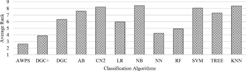
Fig.5. Average rank of the classification algorithms for accuracy.

llllllllllll

AWPS DGC+ DGC AB CN2 LR NB NN RF SVM TREE KNN

Classification Algorithms

Fig.6. Average AUC values.

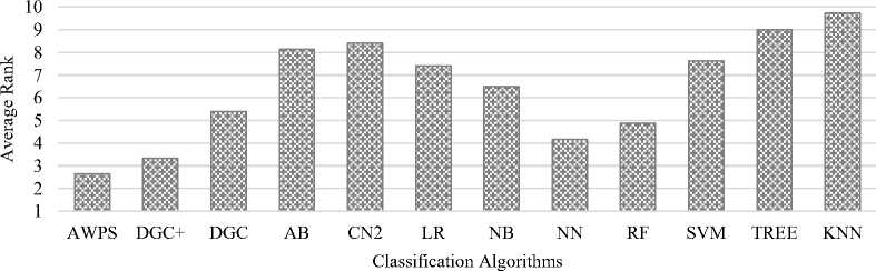
Fig.7. Average rank of the classification algorithms for AUC.

Table 12. Classification AUC Comparison

S.No	Dataset	Classification Algorithms
S.No	Dataset	AWPS	DGC+	DGC	AB	CN2	LR	NB	NN	RF	SVM	TREE	KNN
1	Appendicitis	0.884	0.854	0.835	0.697	0.814	0.797	0.833	0.869	0.786	0.830	0.714	0.798
2	Audiology	0.892	0.889	0.875	0.846	0.869	0.857	0.832	0.850	0.855	0.823	0.874	0.807
3	Australian	0.899	0.886	0.852	0.817	0.883	0.903	0.878	0.934	0.936	0.713	0.812	0.744
4	Balance	0.862	0.875	0.805	0.799	0.805	0.827	0.842	0.887	0.877	0.889	0.816	0.783
5	Breast cancer	0.645	0.647	0.608	0.666	0.597	0.597	0.612	0.684	0.604	0.550	0.587	0.600
6	Bupa	0.699	0.674	0.653	0.650	0.647	0.625	0.651	0.669	0.610	0.602	0.625	0.612
7	Car	0.994	0.998	0.991	0.973	0.908	0.927	0.971	0.981	0.993	0.949	0.897	0.945
8	Charditography	0.999	0.996	0.997	0.992	0.919	0.945	0.987	0.985	0.987	0.991	0.904	0.844
9	Dermatology	0.989	0.991	0.917	0.958	0.932	0.906	0.845	0.990	0.992	0.987	0.874	0.847
10	Ecoli	0.978	0.957	0.951	0.856	0.909	0.922	0.958	0.963	0.957	0.962	0.884	0.945
11	German Credit	0.751	0.743	0.702	0.619	0.672	0.708	0.765	0.749	0.758	0.578	0.650	0.575
12	Glass	0.865	0.854	0.759	0.773	0.814	0.797	0.851	0.853	0.818	0.815	0.807	0.798
13	Haberman	0.698	0.689	0.687	0.608	0.593	0.560	0.690	0.678	0.669	0.559	0.615	0.599
14	Hayes-Roth	0.936	0.948	0.961	0.914	0.904	0.895	0.952	0.946	0.927	0.949	0.902	0.834
15	Hepatitis	0.771	0.763	0.734	0.641	0.782	0.715	0.775	0.760	0.750	0.716	0.677	0.584
16	Ionosphere	0.950	0.931	0.672	0.890	0.714	0.882	0.927	0.960	0.968	0.811	0.836	0.917
17	Iris Plants	0.999	0.994	0.995	0.960	0.887	0.957	0.979	0.987	0.986	0.989	0.878	0.897
18	Lenses	0.891	0.897	0.871	0.824	0.798	0.848	0.857	0.851	0.882	0.874	0.841	0.802
19	Lymphography	0.925	0.923	0.935	0.811	0.877	0.804	0.887	0.945	0.930	0.908	0.793	0.904
20	Monk-1	0.972	0.956	0.945	0.988	0.899	0.716	0.729	0.965	0.979	0.579	0.920	0.894
21	Monk-2	0.970	0.978	0.974	0.890	0.928	0.536	0.534	0.975	0.874	0.492	0.981	0.678
22	Monk-3	0.991	0.988	0.989	0.954	0.945	0.988	0.984	0.982	0.981	0.978	0.969	0.977
23	Mushroom	0.999	0.995	0.996	0.974	0.921	0.994	0.991	0.995	0.994	0.992	0.935	0.927
24	Nursery	0.984	0.979	0.937	0.985	0.983	0.983	0.979	0.984	0.983	0.927	0.978	0.979
25	Phoneme	0.875	0.866	0.851	0.848	0.819	0.812	0.828	0.896	0.889	0.479	0.811	0.879
26	Pima	0.788	0.765	0.741	0.689	0.740	0.726	0.719	0.734	0.781	0.587	0.616	0.738
27	SolarFlare	0.912	0.916	0.929	0.898	0.917	0.939	0.917	0.928	0.921	0.915	0.898	0.899
28	Sonar	0.886	0.891	0.811	0.633	0.692	0.789	0.856	0.879	0.885	0.799	0.721	0.882
29	Soybean	0.999	0.998	0.997	0.948	0.884	0.957	0.968	0.945	0.849	0.988	0.966	0.844
30	Spambase	0.960	0.979	0.980	0.975	0.949	0.961	0.960	0.980	0.982	0.709	0.922	0.877
31	TAE	0.788	0.784	0.765	0.748	0.755	0.635	0.642	0.704	0.798	0.639	0.785	0.619
32	Tic-Tac-Toe	0.878	0.865	0.712	0.832	0.818	0.852	0.748	0.849	0.876	0.864	0.856	0.765
33	Titanic	0.781	0.769	0.772	0.768	0.768	0.759	0.716	0.768	0.766	0.500	0.768	0.656
34	Vehicle	0.871	0.857	0.827	0.805	0.838	0.843	0.809	0.860	0.817	0.895	0.800	0.799
35	Voting	0.990	0.987	0.978	0.933	0.963	0.995	0.972	0.992	0.991	0.979	0.880	0.912
36	Vowel	0.985	0.982	0.979	0.907	0.897	0.946	0.946	0.911	0.981	0.975	0.856	0.811
37	WDBC	0.989	0.987	0.975	0.930	0.859	0.905	0.971	0.975	0.986	0.980	0.902	0.888
38	Wine	0.965	0.973	0.970	0.824	0.834	0.965	0.991	0.987	0.948	0.955	0.889	0.875
39	Yeast	0.996	0.991	0.987	0.972	0.851	0.978	0.885	0.987	0.879	0.954	0.971	0.960
40	Zoo	0.981	0.998	0.935	0.954	0.979	0.989	0.981	0.979	0.980	0.999	0.964	0.845
Average AUC		0.905	0.900	0.871	0.844	0.839	0.844	0.855	0.895	0.886	0.817	0.834	0.813
Average Rank		2.650	3.325	5.400	8.150	8.400	7.400	6.500	4.175	4.875	7.625	9.000	9.725

The average accuracy of the proposed algorithm is higher than other existing algorithms. The average accuracy of AWPS is 88.1% and that of DGC+ is 86.8%. Neural Networks is having equally high performance as DGC+. Ensemble classifiers such as random forest, support vector machine and Adaboost provides better results. The average accuracy is depicted in Fig. 4.

The proposed algorithm provides the first rank for 19 datasets. It takes the first and the second positions for 24 datasets and the top three positions for 29 datasets. The average rank of each algorithm employed in the experimental study for the classification accuracy has been computed. The average rank for the proposed algorithm AWPS is 2.625. The average ranks of DGC+, neural network, and random forest are 3.875, 4.25 and 4.925 respectively. The graph for the average rank is depicted in Fig.5.

The statistical analysis has been carried out for the classification accuracy using ANOVA. The statistical model creates F-distribution with F value = 3.867 and F critical value = 1.809. Thus with the critical difference of 2.508, the results are significant at a 5% significance level. The null hypothesis has been rejected by concluding that there is a difference between the classification accuracy of the algorithms under study.

The performances of the classification algorithms used

in the study are measured using another metric AUC values of AUC for the classification algorithms are which is significant for imbalanced class data [35]. The depicted in Fig.6. values of AUC for all the algorithm and for each dataset The proposed algorithm provides the best result for 17 are calculated and are shown in Table 12. The proposed datasets. It takes the top two positions for 23 datasets and algorithm shows the maximum value for 17 out of 40 the second position for 24 datasets and top three positions datasets. DGC+ classifier and neural networks provide for 27 datasets. The average rank of each algorithm better AUC value. employed in the experimental study for the AUC has The average AUC value for the proposed AWPS been computed. The average rank for the proposed algorithm is 90.5%. The average AUC values for the algorithm AWPS is 2.65. The average ranks of DGC+, DGC+, neural networks, and random forest are neural network, and random forest are 3.325, 4.175 and approximately 90% which are considered as the better 4.875 respectively. The graph for the average rank of performance. However, AWPS perform well and provide AUC is depicted in Fig.7. a better result than the other algorithms. The average Table 13. Evaluation Time Comparison
	Dataset	AWPS (ms)	DGC+ (ms)	DGC (ms)	NN (ms)	RF (ms)	SVM (ms)
	Appendicitis	1.6245	5.1123	3.5426	9.5918	10.3895	7.7856
	Audiology	2.5863	5.2811	2.2255	9.7611	10.5514	8.1425
	Australian	4.5449	8.5507	6.3932	13.0287	13.9218	11.4216
	Balance	4.4541	5.7123	3.8936	10.1921	10.8475	8.5124
	Breast cancer	1.9666	5.6986	3.7708	10.1781	10.6742	8.3462
	Bupa	2.3324	5.6432	3.7519	10.1237	10.8214	8.4212
	Car	5.0563	11.8909	10.1174	16.3707	17.5123	14.7564
	Charditography	6.1256	14.6403	10.4586	19.1174	19.8921	17.5114
	Dermatology	2.1236	9.9809	8.1417	14.4605	15.1473	12.7621
	Ecoli	2.0870	5.7185	4.1192	10.1981	10.1589	8.5779
	German Credit	4.1135	13.1787	9.3940	17.6583	18.9563	15.8754
	Glass	2.0154	5.9765	4.2315	10.4552	11.1289	8.5478
	Haberman	1.9885	5.1919	3.4609	9.6705	10.1596	7.8579
	Hayes-Roth	1.9631	5.0787	3.4939	9.5572	10.3578	7.5124
	Hepatitis	1.9253	5.4077	3.7607	9.8882	10.8476	8.2415
	Ionosphere	3.9431	10.5558	7.8677	15.0289	15.9467	13.3247
	Iris Plants	1.8662	5.1143	3.4446	9.5932	10.4758	7.9912
	Lenses	1.4988	4.8908	3.1446	9.3689	10.2478	7.6452
	Lymphography	1.8315	5.2809	3.5715	9.7587	10.6472	8.0132
	Monk-1	2.8125	5.9141	4.2473	10.3936	11.1425	8.6523
	Monk-2	1.7642	6.6457	4.4919	11.1247	11.8932	9.4124
	Monk-3	1.7479	5.9226	4.2308	10.4021	11.1348	8.4123
	Mushroom	13.8399	26.0123	19.4919	30.4921	31.2617	28.7856
	Nursery	21.0258	114.0142	69.1257	118.4937	119.2163	116.7523
	Phoneme	9.4252	23.0148	17.4606	27.4942	28.2987	25.7123
	Pima	2.4446	10.2452	7.7213	14.7246	15.6124	13.4719
	SolarFlare	4.6582	13.8917	10.6717	18.3709	19.2478	16.7752
	Sonar	2.3467	12.7983	11.2292	17.2777	18.1793	15.5443
	Soybean	2.3178	6.9121	4.6919	11.5913	12.3972	9.6635
	Spambase	10.8023	56.9142	42.4606	61.3930	62.1863	59.6846
	TAE	1.7723	5.2453	3.4934	9.7244	10.6732	8.1247
	Tic-Tac-Toe	2.2632	9.5250	8.8306	14.1143	14.9875	12.3689
	Titanic	6.1236	25.2518	19.4917	29.7317	30.5288	28.1459
	Vehicle	2.1815	12.3209	9.7250	16.9145	17.7349	15.1475
	Voting	1.5567	5.6910	3.9754	10.1723	10.8752	8.2514
	Vowel	1.9256	13.0810	9.4224	17.5647	18.7236	15.2278
	WDBC	2.1201	6.2451	4.2473	10.6243	11.7963	9.2345
	Wine	1.8523	6.3743	4.3708	10.7581	11.9896	9.1856
	Yeast	4.8734	14.2447	9.1424	18.3257	19.4712	17.2256
	Zoo	2.9828	5.6626	2.8718	10.2435	10.2578	9.0789
	Mean Evaluation Time	3.8721	13.1208	9.2544	17.5983	18.4073	15.9026

C. Time Performance

Apart from accuracy and AUC, the evaluation time of the proposed method is also compared with the existing techniques. The computational complexity using Big-O notation for the proposed algorithm is O(nm) where n is the number of records in the datasets and m is the number of attributes selected using proposed attribute score based ranking algorithm. The computation complexity of the other existing algorithms having better classification accuracy or AUC values such as DGC, DGC+, RF, SVM and NN are O(mn ² ), O(mn ² ), O(tmn(log n)), O(n ³ ), and O(n ⁴ ) where n is the number of records and m is the number of attributes. The computational complexity of DGC and DGC+ are same and the complexity of the RF algorithm also depends on the number of trees to be constructed denoted as t. Thus, the proposed algorithm has less computational complexity and thus it is considered faster than other algorithms.

The evaluation time to classify an unlabeled sample using the proposed AWPS algorithm is compared with that of other algorithms such as DGC+, DGC, NN, RF and SVM using the 40 datasets listed in Table 10. The valuation time for all the mentioned algorithms are measured and the values are shown in Table 13. The proposed method has less evaluation time for all the datasets than DGC+, NN, RF and SVM. However, the execution time of AWPS algorithm is less than the DGC algorithm for all the datasets except Audiology, Balance, and Zoo. Also the mean Evaluation time for the proposed AWPS algorithm is 3.87 ms, and for the existing algorithms such as DGC+ is 13.12 ms, DGC is 9.25 ms, NN is 17.6 ms, RF is 18.41 ms and SVM is 15.9 ms. Thus it is found that the proposed AWPS method has less computational time for classifying the datasets.

D. Statistical Analysis and Discussion

The statistical analysis has been carried out for the AUC values of all the methods using ANOVA. The statistical model creates F-distribution with F value = 2.957 and F critical value = 1.809. Thus with the critical difference of 1.148, the results are significant at a 5% significance level. The null hypothesis has been rejected by concluding that there is a difference between the AUC value of the algorithms under study.

On average, the datasets used for the experimental analysis consist of 1312 instances, 16.33 attributes, and 4.5 classes, out of which the proposed algorithm provides better performance in classification accuracy and acquire top 3 positions for 29 among 40 datasets having the average of 1403 instances, 17.3 attributes, and 4.6 classes.

Similarly, the proposed algorithm has a good AUC value than other algorithms and obtains top 3 positions for 27 datasets having mean values as 1412 instances, 16.6 attributes, and 5.15 classes. DGC+, neural networks and ensemble methods provide better accuracy. However, AWPS algorithm provide even better results than other algorithms.

V. Conclusion

In this paper, an average weighted pattern score with attribute rank based feature selection classifier has been suggested for classifying the datasets in an improved way. The proposed feature selection algorithm computes the attribute scores based on their contribution towards better classification. An average weighted pattern score based classification algorithm is suggested for better classification of unlabeled datasets. The main advantage of the proposed AWPS is that its simplicity and better performance than many existing classification methods. The proposed method attained better classification accuracy and AUC values for most of the imbalanced datasets under study when compared with other existing classifiers. The AWPS classification algorithm is well suitable to deal with imbalanced class problem. Statistical analysis were also performed to validate the results obtained from the experiments to support the high performance of the proposal. It is also shown that the evaluation time for the proposed classifier is lower than other significant existing classification algorithms.

Список литературы Efficient classification using average weighted pattern score with attribute rank based feature selection

J. Han, J. Pei and M. Kamber, Data mining: concepts and techniques. Elsevier, 2011.
I. H. Witten, E. Frank, M. A. Hall and C. J. Pal, Data Mining: Practical machine learning tools and techniques. Morgan Kaufmann, 2016.
I. Kononenko and M. Kukar, “Machine Learning and Data Mining: Introduction to Principles and Algorithms,” Cambridge, U.K.: Horwood Publ, 2007.
G. V. Lashkia and L. Anthony, “Relevant, irredundant feature selection and noisy example elimination,” IEEE Trans. Syst., Man, Cybern. B, Cybern., vol. 34, no. 2, pp. 888–897, Apr. 2004.
M. Paliwal and U. A. Kumar, “Neural networks and statistical techniques: A review of applications,” Expert Syst. Appl., vol. 36, no. 1, pp. 2–17, Jun. 2009.
G. Lin, C. Shen, Q. Shi, A. Van den Hengel and D. Suter, “Fast supervised hashing with decision trees for high-dimensional data,” in Proc. of IEEE Conference on Computer Vision and Pattern Recognition, pp. 1963-1970, 2014.
T. R. Patil and S. S. Sherekar, “Performance analysis of Naive Bayes and J48 classification algorithm for data classification,” International journal of computer science and applications, 6(2), pp. 256-261, 2013
D. W. Aha, D. Kibler, and M. K. Albert, “Instance-based learning algorithms,” Mach. Learn., vol. 6, no. 1, pp. 37–66, Jan. 1991.
M. Muja. and D. G. Lowe, “Scalable nearest neighbor algorithms for high dimensional data,” IEEE Transactions on Pattern Analysis & Machine Intelligence, pp. 2227-2240, 2014.
I. Naseem, R. Togneri. and M. Bennamoun, “Linear regression for face recognition,” IEEE transactions on pattern analysis and machine intelligence, 32(11), pp. 2106-2112, 2010.
A. Y. Ng and M. I. Jordan, “On discriminative vs. generative classifiers: A comparison of logistic regression and naive bayes,” Advances in neural information processing systems, pp. 841-848, 2002.
P. G. Espejo, S. Ventura, and F. Herrera, “A survey on the application of genetic programming to classification,” IEEE Trans. Syst., Man, Cybern. C, Appl. Rev., vol. 40, no. 2, pp. 121–144, Mar. 2010.
T. G. Dietterich, “Ensemble methods in machine learning,” International workshop on multiple classifier systems, Springer, Berlin, Heidelberg, pp. 1-15, June 2000.
A. Liaw and M. Wiener, “Classification and regression by random Forest”, R news, 2(3), pp.18-22, 2002.
T. K. An and M. H. Kim, “A new diverse AdaBoost classifier,” in Proc. of Artificial Intelligence and Computational Intelligence (AICI), IEEE, vol. 1, pp. 359-363, 2010.
S. W. Lin, Z. J. Lee, S. C. Chen and T. Y. Tseng, “Parameter determination of support vector machines and feature selection using simulated annealing approach,” Appl. Soft Comput. 8, pp. 1505–1512, 2008.
A. Frank and A. Asuncion, “UCI machine learning repository”, Univ. California, School Inf. Comput. Sci., Irvine, CA. [Online]. Available: http://archive.ics.uci.edu/ml/citation_policy.html
J. Alcalá-Fdez, A. Fernandez, J. Luengo, J. Derrac, S. García, L. Sánchez and F. Herrera, “KEEL data-mining software tool: Data set repository, integration of algorithms and experimental analysis framework,” J. Multiple-Valued Logic Soft Comput., vol. 17, pp. 255–287, 2011.
J. V. Tu, “Advantages and disadvantages of using artificial neural networks versus logistic regression for predicting medical outcomes,” Journal of clinical epidemiology, 49(11), pp. 1225-1231, 1996.
S. Dreiseitl and L. Ohno-Machado, “Logistic regression and artificial neural network classification models: a methodology review”, Journal of biomedical informatics, 35(5-6), pp. 352-359, 2002.
S. S. Nikam, “A comparative study of classification techniques in data mining algorithms,” Oriental Journal of Computer Science & Technology, 8(1), pp.13-19, 2015.
D. L. Poole and A K. Mackworth, “Artificial Intelligence: foundations of computational agents,” Cambridge University Press, 2010.
S. J. Press and S. Wilson, “Choosing between logistic regression and discriminant analysis,” Journal of the American Statistical Association, 73(364), pp. 699-705, 1978, 1978.
Leo Breiman, “Random Forests,” in Machine Learning, 45(1), pp. 5-32, 2001.
J. R. Quinlan, “Bagging, Boosting, and C4.5,” in Proc. of national conference on artificial intelligence, pp. 725–730.
S. C. Chen, S. W. Lin, S. Y. Chou, “Enhancing the classification accuracy by scatter-search-based ensemble approach,” Appl. Soft Comput. 11, pp. 1021–1028, 2011.
K. Ming Leung, “K-Nearest Neighbor Algorithm for Classification,” Polytechnic University Department of Computer Science/Finance and Risk Engineering, 2007.
B. Li, Y. W. Chen, and Y. Q. Chen, “The nearest neighbor algorithm of local probability centers,” IEEE Trans. Syst., Man, Cybern. B, Cybern., vol. 38, no. 1, pp. 141–154, Feb. 2008.
L. Peng, B. Peng, Y. Chen, A. Abraham, “Data gravitation based classification,” Inf.Sci. 179, pp. 809–819, march 2009.
J. Wang, P. Neskovic, and L. N. Cooper, “Improving nearest neighbor rule with a simple adaptive distance measure,” Pattern Recognit. Lett., vol. 28, no. 2, pp. 207–213, Jan. 2007.
Y. Zong-Chang, “A vector gravitational force model for classification,” Pattern Anal. Appl., 11, pp.169–177, May 2008.
A. Cano, A. Zafra, S. Ventura, “Weighted data gravitation classification for standard and imbalanced data,” IEEE Trans. Cybern. 43, December 2013.
N.K. Sreeja, and A. Sankar, “Pattern matching based classification using ant colony optimization based feature selection,” Applied Soft Computing, 31, pp.91-102, 2015.
G. Hesamian, “One-way ANOVA based on interval information,” International Journal of Systems Science, 47(11), pp .2682-2690, 2016
V. López, A. Fernandez, S. Garcia, V. Palade and F. Herrera, “An Insight into Classification with Imbalanced Data: Empirical Results and Current Trends on Using Data Intrinsic Characteristics,” Information Sciences, 250, pp. 113-141, 2013.

Еще

Статья научная