Efficient method of calculating layered conical shells with Lagrange multigrid elements use

Introduction. The layered conical shells (LCS) are widely applied in the space-rocket and aircraft technology. Unlike cylindrical shells, LCS geometrical and stiffness properties depend on axial coordinate that creates great difficulties during analytical and numerical research of the stress strained state (SSS) of such shells..

Since during shells numerical calculations there is no unified approach suitable for the entire range of shell constructions in use, further research in the field of shells computing mechanics is being continued now. In recent years new numerical methods for LCS calculation have been developing and the existing methods have been improving. The method of differential quadratures developed for the solution of the linear and non-linear equations in partial derivatives [1] is applied to the LCS analysis with the equations of the three-dimensional elastic theory use in conic coordinates [2]. In works [3–5] the method of reference surfaces which is used for calculation of multilayer shells and plates is offered for homogeneous and layered shells in a spatial setting calculation. Movements in shell thickness are approximated by means of Lagrange polynomials, and movements in reference surfaces are set by functions which meet boundary conditions. For calculation of layered conical and cylindrical shells the method of discrete singular convolution is used [6]. At the same time only thin shells which deformation submits to Kirkhgofa-Lyava kinematic hypothesis are considered. The method of finite element (MFE) is the most widespread numerical method when calculating shells. The review of works on calculation of composite shells by means of MFE is provided in [7]. Various options of finite elements (FE) are applied to LCS calculation. For example, in work [8] a curvilinear 4-node FE with 20 degrees of freedom for the bearing layers of a 3-layer shell is used, and a filler interlayer is considered in the elastic theory threedimensional setting. In work [9] the layered conical structures of a shell for bends with the use of isoparametric FE and high order displacement deformation models are analysed.

The increased requirements to modern shell constructions cause the necessity of algorithms of approximate solutions tasks of the elastic theory with the given small error development and improvement. It is difficult to apply the known approaches from the theory of materials strength, or the two-dimensional elastic theory based on the simplifying hypotheses that often leads to a bigger error of the achieved results to obtain such solutions. In this regard there is a need for the development of such FE in which the deformation of a composite shell is considered in three-dimensional setting taking into account its structure without simplifying kinematic and static hypotheses introduction. In works [10; 11] the computational method of composite circular cylindrical shells in a three-dimensional setting with application of multigrid FE (MGFE) in which movements are approximated by means of Lagrange polynomials of various orders is offered.

In this work the numerical computational method of LCS of various form and thickness at the arbitrary static loading in which three-dimensional curvilinear shell type Lagrange MGFE are used is described. The characteristic feature of the MGFE constructing offered procedure is that Lagrange polynomials nodes coincide in shell thickness with MGFE large grids nodes lying on the common borders of multi-module layers. The offered method provides the uniform and fast convergence of approximate solutions that allows to make solutions with the specified (small) error. The effectiveness of the offered MGFE is that they generate discrete models which dimension is several orders less than dimensions of basic models. Examples of calculations are given.

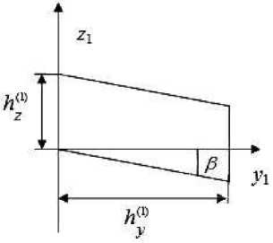
Construction of single-grid FE for conical shell basic model. We will briefly consider the procedure of constructing curvilinear homogeneous single-grid FE (SGFE) construction which create a conic shell basic discrete model on the example of FE V(1) of the 1st order (fig. 1). The procedure of SGFE construction for cylindrical shells at approximation of fields of movements by degree polynomials is explicitly explained in work [12]. Let us consider that FE order is defined by order of a degree polynomial or a Lagrange polynomial constructed on its nodal grid, and the superscript in the symbol corresponds to the nodal grids quantity in an element. SGFE represents a part of the conical shell with the reference sizes hXWhX*2) x h^1 x h^X1) located in a local Cartesian coordinate systemO1x1y1z1 . In fig. 1 designations are introduced: z1O1 y1 – a plane of symmetry, cd - a longitudinal axis of a conical shell, a -FE V(1) corner angle, hz(1) – thickness, hy(1) – length (height), hX*) = aRi (i = 1,2), R1, R2- radiuses of a shell bottom face at FE end faces, P - shell conicity angle, nodes in the drawing are noted by points. Movements, deformations and tension in SGFE V (1) satisfy to the equations of the three-dimensional elasticity theory, recorded in the local Cartesian coordinate systemO1x1y1z1 .

Taking into account that FE reference sizes are small for minor basic splits, we use 1st order polynomials for approximation of movements functions _u (1)_{, v} (1)_{, w} (1) of element V ⁽¹⁾

u ⁽¹⁾, v ⁽¹⁾, w ⁽¹⁾ = a 1 + a ₂ x + a 3 y 1 + a 4 z 1 + a 5 x y 1 + + a 6 z 1 x 1 + a 7 z 1 y 1 + a ₈ x 1 y 1 z 1 .               (1)

The total potential energy of FE V ⁽¹⁾ in a matrix form is the following [13]

П⁽¹⁾ ( 6 ⁽¹⁾) = ¹J ( 8 ⁽¹⁾) T ( B ⁽¹⁾) T DB ^<1) 8 ^<1) dV - 2 _V

- J ( 8 ⁽¹⁾) T (№ ) ) T F ⁽¹⁾ dV - J ( 6 ⁽¹⁾) T (№)) T q^{G )} dS ,     (2)

VS where B(1) , D – matrixes of deformations and elastic modules V (1) ; F(1) , q(1) – vectors of volume and surface forces; δ(1) , N(1) – a vector of nodal unknowns and a matrix of form functions; V , S – FE V (1) area and surface; T – transposition.

From д П^<1)( 8 ^<1)) / 9 8 (1) = 0 condition we find formulas for calculation of a stiffness matrix K ⁽¹⁾ and a nodal forces vector P ⁽¹⁾ in the local coordinate frame O ₁ x ₁ y ₁ z ₁

K ^G) = J ( B^{G )}) T DB ⁽¹⁾ dV ,

V

P^{G )} = J ( N ⁽¹⁾) T F ⁽¹⁾ dV - J (№) ) T q ⁽¹⁾ dS .       (3)

V

S

Let us note that the continuity of movements on FE curvilinear borders V ⁽¹⁾ (fig. 1) is broken. However, as it is well-known [14], realization of continuity of movements on borders of curvilinear FE is not a necessary condition for convergence of numerical solutions to precise and is checked in each case. The carried out numerical experiments show that at curvilinear homogeneous FE V ⁽¹⁾ reference sizes decrease numerical solutions converge to precise.

In (3) we define integrals numerically. Let us present area V by elementary curvilinear subareas V ¹,..., V^N ,

∪ N _n

Vⁿ , N – total number of subareas. For n = 1

V” area let us introduce designations: A z = h® / m 1 , A y = h ^G) / m ₂, Aa = a / m 3 , Aa - corner angle of area

V ⁿ ; m ₁ , m ₂ , m ₃ – the given integral numbers;

N = m 1 m ₂ m 3 .

The form of area V n is a part of the truncated conical shell with thickness h (Az = h / cos P), height Ay and corner angle Aa . Let us note that areas V” (irrespective of their sizes) geometrically precisely represent FE V (1) curvilinear area. Let x1n , y1n , z1n – area V n gravity centre coordinates in the local coordinate system O1 x1 y1 z1. The volume A Vn of area V” is defined by the approximate formula A Vn = Az AyAa Rn, where Rn -distance from a cone axis to an area V n gravity centre. Matrix B(1) , which elements are calculated for values of coordinates x1n , y1n , z1n , let us designate B(1) (x1n , y1n ,z1n ) . We approximately find a stiffness matrix K(1) by virtue to (3) on a formula

N

• (1)               (1) n n n T (1) n n n

^K / _x ^{( B ( x} 1 , ^y 1 , ^z 1 )) DB ^{( x} 1 , ^y 1 , ^z 1 ^{) A} V ” . ⁽⁴⁾ ” = 1

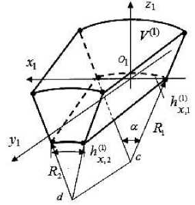
Fig. 1. Homogeneous FE V ⁽¹⁾ ( V_n ⁽¹⁾ ) ( a ), the cross section of the FE plane z ₁ O ₁ y ₁ ( b )

b

Рис. 1. Однородный КЭ V ⁽¹⁾ ( V_n ⁽¹⁾ ) ( а ), сечение КЭ плоскостью z ₁ O ₁ y ₁ ( б )

The vector of nodal forces P ⁽¹⁾ of element V ⁽¹⁾ is also defined numerically.

The differences of the offered curvilinear SGFE V ⁽¹⁾ construction procedure from isoparametric FE construction [13] are as follows. Isoparametric FE use is proved by the necessity of FE stiffness matrix calculation simplification. Curvilinear coordinates are transformed to rectilinear (Cartesian) coordinates, and curvilinear FE is transformed in rectilinear (two – three-dimensional) by the equivalent transformations. Herewith stiffness matrix numerical calculation assumes the known quadrature formulas use [14]. Transformation of curvilinear coordinates demands calculation of a straight line and an inverse Jacobi matrix in each calculated point at a numerical integration.

The offered option of SGFE stiffness matrix calculation (3), (4) is simpler and has the following advantages:

– curvilinear FE V ⁽¹⁾ is projected in the local threedimensional Cartesian coordinate system and therefore there is no need to define a straight line and an inverse Jacobi matrix [13; 14] that is required when using isoparametric FE;

– when constructing approximating displacement functions u ⁽¹⁾ , v ⁽¹⁾ , w ⁽¹⁾ FE V ⁽¹⁾ we use the known degree polynomials of the 1st, 2nd and 3rd orders [13] which are recorded in local Cartesian coordinate systems which do not contain FE rigid displacement. In case of local curvilinear coordinate frames at constructing curvilinear shell FE application there is a need to construct such approximating functions of movements in which FE rigid displacements are excluded that is connected with particular difficulties [15];

– the numerical integration is performed according to the simplest formula when in each partial area V ⁿ the value of function is chosen constant and equal to the value of function in a gravity centre of this area. At decrease of the partial areas sizes the value of a FE V ⁽¹⁾ stiffness matrix in a limit converges to precise value.

Procedures of the 2nd, 3rd order SGFE construction which geometrically are similar to the FE V ⁽¹⁾ form (fig. 1) are similar to the above described.

Further we will consider the construction of MGFE with ideal connections between the heterogeneous structure components in case of movements approximation by Lagrange polynomials on the example of three-grid FE (ТGFE) V ⁽³⁾ . Such element consists of M two-grid FE (TGFE) V_m ⁽²⁾ , ( m = 1,..., M ), each one is composed from N homogeneous SGFE V n ⁽¹⁾ ( n = 1,..., N ).

Construction of two-grid FE for a conical shell. Let us consider the procedure of multilayer TGFE for a conical shell construction on the example of tree-layer TGFE V (2) of the 3rd order in its thickness which is used when calculating a 3-layer conical shell in thickness h with the reference sizes hx(,21) (hx(2,2))× hy(2) ×h located in the local Cartesian coordinate system O2x2y2z2 (fig. 2). In case of calculating a k-layer conical shell it is necessary to use k- layer Lagrange TGFE of a k-order in thickness.

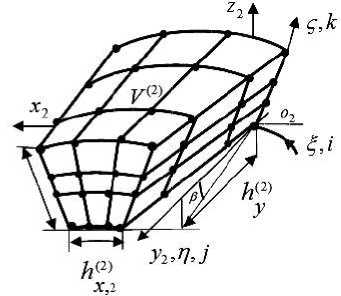
Fig. 2. Three-Layer TGFE V ⁽²⁾ ( V_m ⁽²⁾ )

Рис. 2. Трехслойный ДвКЭ V ⁽²⁾ ( V_m ⁽²⁾ )

SGFE nodes V_n ⁽¹⁾ , n = 1,..., N , make a fine curvilinear grid on which TGFE large grid is constructed. Let us note that large grid nodes on shell thickness lie on the common borders of TGFE multi-layers which generally have various thicknesses. Lagrange polynomials construction in the local curvilinear coordinate frame O ₂ ξης on TGFE large grid for cylindrical shells is considered in [10; 11] and can be applied to LCS calculation. The basic function N_ijk for node P ( i , j , k ) (fig. 2) in curvilinear coordinates α , η , ζ is N_ijk ( α , η , ζ ) = L_i ( α ) L_j ( η ) L_k ( ζ ) , where L_i ( α ) , L_j ( η ), L_k ( ζ ) – Lagrange polynomials:

Li(α)= ∏n1 α-αn , Lj(η) = ∏n2 η-ηn , n=1,n≠iαi- αn              n=1,n≠jηj -ηn n3

L k ( ζ ) = ∏ ^{ζ ζ n} .                (5)

n = 1, n ≠ k ζ k ^- ζ n

Using designations u_i ⁽²⁾ , v_i ⁽²⁾ , w_i ⁽²⁾ , N_i ⁽²⁾ for movements and form functions of TGFE i node in the coordinate frame O ₂ x ₂ y ₂ z ₂ , movements functions u ⁽²⁾, v ⁽²⁾, w ⁽²⁾ can be given as [13]

n0

u(2) = ∑Ni(2)ui(2)    , v(2)=∑Ni(2)vi(2) , i=1

n ₀

w(2) =   N (2)w(2) , n = n n n .(6)

i i 0123

i = 1

We will record the functional of the total potential energy П⁽²⁾ for basic TGFE V ⁽²⁾ split as follows

N

П⁽²⁾ = ∑ (¹( δ ⁽ n ¹⁾) ^T K ⁽ n ¹⁾ δ ⁽ n ¹⁾ - ( δ ⁽ n ¹⁾) ^T P n ⁽¹⁾),         (7)

n = 1 ²

where K ⁽ _n ¹⁾ – stiffness matrix, P _n ⁽¹⁾ , δ ⁽ _n ¹⁾ – vectors of nodal forces and movements of SGFE V_n ⁽¹⁾ which correspond to the coordinate frame O ₂ x ₂ y ₂ z ₂ .

The use of small splits generates TGFE with a large number of nodal unknowns. For decrease in TGFE dimension the following procedure is used. By means of functions (6) we present the vector of nodal movements 6® of SGFE V n ⁽¹⁾, n = 1,..., N through the vector of nodal movements δ ⁽²⁾ of TGFE V ⁽²⁾ . As a result, we receive equality

6^ ’ = А П ²⁾ 6 ( ²⁾, (8)

where A n²’ - a rectangular matrix, n = 1,..., N .

Substituting (8) in (7) and, following the principle of the total potential energy minimum, i. e. д П < ²⁾( 6 < ²⁾)/ д 6 ( ²⁾ = 0, for TGFE V ( ²⁾ we get the ratio K ⁽²⁾ 6 ⁽²⁾ = p ⁽²⁾ defining its an equilibrium state where

NN

K ⁽²⁾ = 2 ( А П ²⁾) T K« А П ²’ , P ⁽²⁾ = 2 ( А П ²’) ^T P n ^G), (9) n = 1 n = 1

K ⁽²⁾ – stiffness matrix, P ⁽²⁾ – vector of nodal forces TGFE V ⁽²⁾ .

Procedures of constructing composite Lagrange TGFE of p – order construction, geometrically similar to TGFE V ⁽²⁾ (fig. 2), with application of Lagrange polynoms of p -order, are similar to the considered procedure.

The calculations show that at increase in dimensions of TGFE basic splits time expenditure on construction of matrixes K ⁽²⁾ and P ⁽²⁾ according to formulas (9) significantly increases. In this case it is expedient to apply ThrGFE which constraction requires less time expenditure and which generate shells discrete models of smaller dimension, than TGFE.

Construction of three-grid FE for a conical shell. We will consider the procedure of multilayer ThrGFE for a conical shell construction we will consider on the example of 3-layer ThrGFE V ⁽³⁾ of the 3rd order in its thickness with the reference sizes h ;1 ( h ³ ’ ) x h^' x h , disposed in the local Cartesian coordinate system O ₃ x ₃ y ₃ z ₃ . ThrGFE has the form similar to TGFE shown in fig. 2. For ThrGFE the order of Lagrange polynomials on coordinates x ₃ , y ₃ can be arbitrary, different from the polynomials order on these coordinates in TGFE. ThrGFE has the 3rd order in its thickness h (coordinate z ₃ ) which is used when calculating 3-layer conical shells. In case of a m -layer conical shell calculation it is necessary to use a m -layer Lagrange ThrGFE of m order in thickness.

The ThrGFE area consists of M TGFE V_m ⁽²⁾ , m = 1,..., M which geometrically precisely represent the ThrGFE area. The TGFE nodes, included in ThrGFE, generate a curvilinear grid on which a ThrGFE large grid is being constructed. Let us note that ThrGFE large grid nodes, as well as in case of TGFE lie on the common borders of multi-layers which generally have various thickness. The total potential energy П⁽³⁾ of ThrGFE V ⁽³⁾ is represented by

M

• (3)            ¹     (2) T (2)    (2)        (2) T (2)

^П = 2 ⁽T^{( 6} m ’ ^K m ⁶ m — ^{( 6} m ’ ^P m ’,    ⁽¹⁰⁾

m = 1 ²

where δ ⁽ _m ²⁾ – a nodal movements vector; K ⁽ _m ²⁾ , P _m ⁽²⁾ – a stiffness matrix and a nodal forces vector TGFE V_m ⁽²⁾ , which correspond to the coordinate frame O ₃ x ₃ y ₃ z ₃ , m = 1,..., M .

Movements functions u(3), v(3), w(3) ThrGFE V(3) , constructed on a large grid by means of Lagrange polynomials, we will present as p0

u <3 = У N(3) u (3),   v(3) = У N(3) v<3), iiii i=1

p ₀

w <3 =2 Nf) w^,(11)

i = 1

where u_i ⁽²⁾ , v_i ⁽²⁾ , w_i ⁽²⁾ , N_i ⁽²⁾ u_i ⁽³⁾ , v_i ⁽³⁾ , w_i ⁽³⁾ , N_i ⁽³⁾ – movements and an i node form function of a ThrGFE large grid in the coordinate frame O ₃ x ₃ y ₃ z ₃ ; p ₁, p ₂, p ₃ – ThrGFE Lagrange polynomials orders on coordinates x 3 , У 3 , z 3 , P 0 = P 1 P 2 P 3 .

For decrease in number of ThrGFE nodal unknowns the vector of FE Vm(2) nodal movements δ(m2) by means of (11) we present through the FE V (3) vector of nodal movements δ(3) . As a result, we obtain equality sm2)=Am3)6<3),                    (12)

where A m ³ ) - a rectangular matrix, m = 1,..., M .

Substituting (12) in (10) and, minimizing a functional П⁽³⁾ on movements δ ⁽³⁾, for ThrGFE V ⁽³⁾ we receive a matrix ratio K ( ³⁾ 6 ( ³⁾ = p ( ³⁾ which corresponds to its equilibrium state, where

MM

K ( ³⁾ = 2 ( A m ?) ) T K m 2) A m ?) , P ( ³⁾ = 2 ( A m ?’ ) T P m ² . (13) m = 1                                   m = 1

where K ⁽³⁾ , P ⁽³⁾ – a stiffness matrix and a nodal forces vector of ТhrGFE V ⁽³⁾ .

Remark 1. The dimension of a vector δ ⁽³⁾ (i. e. dimension of ThrGFE V ⁽³⁾ ) does not depend on TGFE V_m ⁽²⁾ total number included in ThrGFE. Therefore, ThrGFE splitting into TGFE V_m ⁽²⁾ and SGFE V_n ⁽¹⁾ can be arbitrarily small that allows to consider a complex heterogeneous structure and a form of ThrGFE V ⁽³⁾ .

Remark 2. The quantity of TGFE layers can be less than the number of shell layers. For example, when constructing a 6-layer ThrGFE it is possible to use 3-layer TGFE (fig. 2) or 2-layer TGFE. As the calculations show, it leads to decrease in time expenditure with an insignificant change of solution error.

The calculations show that the arrangement of ThrGFE large grid nodes on borders of multi-layers provides the uniform and fast convergence of approximate solutions.

Using ThrGFE, according to the procedure similar to p. 3, we construct 4-grid FE, and k -grid FE, k >  4 . Let us note that k -grid FE generate discrete models of conical shells of smaller dimension, than ( k - 1) -grid FE. The proposed method can be used for calculation of multilayer conical shells with layers of various thickness.

Results of numerical experiments

Example 1. Let us consider a 4-layer elastic console conical shell under the influence of external pressure q in the Cartesian coordinate system Oxyz , y -axial coordinate, h - thickness, L - shell length. At y = 0 a shell is rigidly restrained. At shell end faces the radiuses of a median surface are equal to R at y = 0 and r at y = L, p - cone angle. Shell layers are isotropic homogeneous bodies. Top and bottom layers have thickness h / 6 , two internal layers –h /3 . Young’s modules of 4 layers (starting with internal) are respectively equal: 10E; 3E; 5E; 20E , E – an elastic module, v - Poisson’s ratio. The reference points B and С on the external surface of the shell lie on the crossing of the plane Oyz and transverse sections y = L /2; L . In calculations 1/4 part of the shell is used. Basic discrete models of the Rn0 shell consist of the 1st order homogeneous SGFE Vn(1) with the reference sizes h*: \( h ’,2) x h’ x h’, hhXj n , h£’ = hyl)/ n , h’ = hZ!)/ n , n = 1,...,5, j = 1,2,                 (14)

j = 1 corresponds to Vn11 size on the circumferential coordinate at a larger FE end face, j = 2 - at a smaller end face Vn(1) . The fine grid dimension of model Rn0 for 1/4 shell part is determined according to formulas mn = 324n +1, m^ = 324n +1,

m ; 3 = 12 n + 1, n = 1,...,5,           (15)

where m ¹ _n – a grid dimension in the shell tangential direction, m_n ² – in axial, m_n ³ – in radial.

On basic models R0, n = 1,...,5, we project multigrid discrete models of the Rn shell which consist of Lagrange ThrGFE size 81 h**’l(h**’2) x 81 hx h s. ThrGFE consist xn,1 xn,2          yn of Lagrange TGFE with sizes 9h(‘’Jh**’2)x9hЯ? x h. xn,1 xn,2         yn

Lagrange polynomials are used in ThrGFE, which are defined by formulas (5) which in local coordinates have the third order in the tangential and axial direction and the fourth order – in radial that corresponds to quantity of layers in the shell. In discrete models R_n TGFE and ThrGFE large grids nodes lie on the common borders of heterogeneous layers in shell thickness.

The results of calculations for discrete models R_n at the following values of parameters are given in tab. 1: L = h ₀; R = h o ; r = 0,6 h „ ; h = 0,06 h „ ; q = - 0,5 q o ;

h ₀ = 1 m; E = 1 h Pa; q ₀ = 1 MPa; v = 0,3; p = 21,8⁰. Designations are introduced in tab. 1: w = w, /⁽ q o ^h o E ^{- 1 )} , ^g * * ^g n / q o , где w n , ^g * ^{- the di}mensionless normal movements and the equivalent stresses (for the model R_n reference points B and С ). We determine stresses g * according to the 4th theory of strenght. We get values 5_{n n} (%), 5 _wn (%) by the formulas

• 5 . n (%) = 100% x | g * -g * - 1 |/ g * ,

5 w , n (%) = 100% X | w * - w n — 1 |/ w * , n = 2,...,5. (16)

The nature of sizes 5 _{w n} (%), 5 . _n (%) change shows fast convergence of stress g * and movements w * . As for model R ₅ the values 5 _{w 5}(%) _B = 0,0049, 5 _{w 5}(%) C = 0,0232 and values 5_{g 5}(%) _b = 0,0272, 5_{g 5}(%) c = 0,007 are small, from the point of view of engineering practice it is possible to consider that movements ( w 5 ) _B =- 0,82302, ( w * ) C =- 0,3879 and stresses ( g * ) _b = 17,49340 , ( . 5 ) С = 11,6266 in the conical shell reference points B and C are calculated with a small error (less than 0,3 %).

The comparison of the results received by means of ThrGFE (grid1621 x 1621 x 61), by means of SGFE (grid163 x 163 x 13) received in the ANSYS program complex (PC) and by means of FE for a two-dimensional task of the elasticity theory [13] is given in tab. 2. We will consider the numerical results received by means of twodimensional axisymmetric task statement [13] the most precise within MFE. The smallest error (less than 0,04 %) for the field of movements in the reference points B and C is also provided by ThrGFE. For the equivalent stresses the error is less than 1,2 % for calculation in PC ANSYS, and less than 0,4 % when using ThrGFE. SGFE define movements with an error less than 0,2 % and the stress with an error about 4 % on the free end of a conical shell. The grid size for SGFE exhausts the memory capacity used by electronic computing machine (ECM) that limits the possibility of constructing sequence of solutions by means of SGFE.

The basic discrete model R ₅⁰ dimension (for 1/4 part of a shell) is 480364020 (approximately 0,48 x 10 9 of nodal unknowns), MFE SLAE film width – 296710. The R ₅ multigrid model has 54300 nodal unknowns, MFE SLAE film width is 2775. Realization of MFE for R ₅ multigrid model reduces the order solved by MFE SLAE in 8,8 x 10³ times and demands in 0,96 x 10⁶ times less ECM memory capacity than for the basic model R ₅⁰ in which only SGFE are used. The quantity of ThrGFE (400 ThrGFE) used for calculation in discrete model R ₅ is 14,6 times less than the quantity of FE in PC ANSYS (5850 FE). Thus, ThrGFE use when calculating SSS allows to save significantly ECM resources in comparison with PC ANSYS and when using SGFE.

Example 2. Let us consider a conical shell with geometrical sizes and physical properties from example 1 in which two identical cutouts are located symmetrically relatively the planes Oyz and Oxy , with the length l and a cone angle α = π /4 , 4 l – the length of a frustum of a cone on the generatrix (fig. 3).

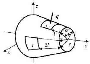
Fig. 3. Shell design scheme

Рис. 3. Расчетная схема оболочки

Standard pressure of the distributed load q = - 0,5 q ₀ , q ₀ = 1 MPa is enclosed on the area of the shell upper face 0,5 L ≤ y ≤ 0,75 L and a cone angle of a loading area γ = π / 2 symmetrically concerning the plane Oyz . In calculations we use a half of a shell.

In calculation the same basic discrete models and Lagrange TGFE and ThrGFE as in example 1 are used. The results of calculations for discrete models R_n ( n = 1,..., 7 ) are given in tab. 3. The nature of values change δ _{w , n} (%) , δ_{σ , n} (%) shows fast convergence of the equivalent tension σ _n and normal deflections w_n .

As for R7 model deflections values δw,7 (%)B = 0, 025 , δw,7(%)C = 0, 030 and values of stre-ses δσ,7 (%)B = 0,1098 , δσ,7(%)C = 0, 0178 are small, it is possible to consider that movements (w7*)B = -1, 07661 , (w7*)C = -1,13964 and stresses (σ*7)B = 10, 01830 , (σ*7)B = 0, 61903 in the reference points B and C of LCS are calculated with a small error (about 0,03 % and 0,11 % respectively) that is considered to be an acceptable result from the point of view of engineering practice.

Comparison of these results with the results of task calculation is carried our in PC ANSYS. The dimensionless values of the equivalent stresses σ ⁰ and normal movements w ⁰ in points B and C received in PC ANSYS are σ ⁰ = 9,952, σ ⁰ = 0, 638 and w ⁰ = - 1, 091 . BC  B

The relative accuracies of a deviation of movements and stresses values in points B and C received in R ₇ discrete model when using ThrGFE from the results received in PC ANSYS are less than 1,2 % for movements and less than 3 % for stresses.

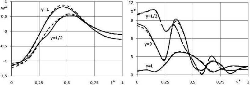
In fig. 4 distributions on an external surface of a conical shell of the dimensionless normal movements ( w ^* = w ₅^* ) in sections y = L /2; L and the equivalent stresses ( σ ^* = σ ^*₅ ) in sections y = 0; L / 2; L depending on the parameter s ^* = s / P , s – distance from an axis Oz to a point on an external surface of a shell, P – perimeter of a shell cross section half are shown.

Calculation of SSS is carried out by means of ThGFE for R ₇ model (solid line) and by means of PC ANSYS (dashed line). In all chosen sections of the composite shell construction it is possible to observe the coincidence of SSS, accepted in engineering calculations, received by means of ThGFE and PC ANSYS.

Thr basic discrete model R ₇⁰ dimension (for 1/2 of the shell) is 2460017130 (approximately 2,46 × 10⁹ nodal unknowns), the width of MFE SLAE film – 578601. The multigrid model R ₇ has 199800 nodal unknowns, the width of MFE SLAE film is equal to 3840. Realization of MFE for the multigrid model R ₇ reduces the order of the solved MFE SLAE by 12312 times and demands 1,855 × 10⁶ times less than CEM memory capacity than for the basic model R ₇⁰ in which SGFE are used. The ThGFE quantity used for calculation in discrete model R ₇ (240 FE) is 35 times less than FE quantity used when calculating in PC ANSYS (8436 FE).

Тable 1

The sequence of solutions for a 4-layer conical shell

R n	( wn *) B ( wn *) C	δ w , n (%) B δ w , n (%) C	( σ * n ) B ( σ * n ) C	δσ , n (%) B δ σ , n (%) C
R 1	–0.82538 –0.39056	–	17.41062 11.69263	–
R 2	– 0.82341	0.2392	17.46738	0.3249
	–0.38867	0.4863	11.64802	0.3830
R 3	– 0.82313	0.0340	17.48087	0.0772
	–0.38817	0.1288	11.63100	0.1463
R 4	– 0.82306	0.0085	17.48864	0.0444
	–0.38799	0.0464	11.62579	0.0448
R 5	– 0.82302	0.0049	17.49340	0.0272
	– 0.38790	0.0232	11.62660	0.0070

Тable2

Comparison of calculations results received in different variants of solution

The sequence of solutions for a 4-layer conical shell with cutouts

b

а

Fig. 4. Distribution of deflections w ^* ( a ) and stresses σ ^* ( b ) on the upper surface of the shell in cross sections: y = L ; L / 2;0 . ThrGFE – solid line, ANSYS– dashed line

The method of task solutuion	* w B	* w C	* σ B	* σ C
	δ w (%) B	δ w (%) B	δ σ(%) B	δ C (%) С
ThrGFE	– 0.82302 0.0255	– 0.38790 0.0387	17.49340 0.3787	11.62660 0.0119
SGFE	– 0.82153 0.1556	– 0.38751 0.0619	17.38464 0.2454	12.04767 3.6093
PC ANSYS	– 0.82329 0.0583	– 0.38871 0.2476	17.447 0.1125	11.760 1.1354
[13]	– 0.82281	– 0.38775	17.42740	11.62798

Table 3

R n	R 1	R 2	R 3	R 4	R 5	R 6	R 7
( wn *) B	–1.07084	–1.07250	–1.07441	–1.07539	–1.07597	–1.07634	–1.07661
δ w , n (%) B	–	0.155	0.178	0.091	0.054	0.034	0.025
( wn *) С	–1.12031	–1.13299	–1.13632	–1.13782	–1.13865	–1.13918	–1.13954
δ w , n (%) С	–	1.119	0.293	0.132	0.073	0.047	0.030
( σ * n ) B	9.65343	9.82601	9.92132	9.96536	9.99092	10.00730	10.01830
δ σ , n (%) B	–	1.756	0.607	0.442	0.256	0.164	0.110
( σ * n ) C	0.69330	0.63057	0.62157	0.61965	0.61926	0.61914	0.61903
δ σ , n (%) C	–	9.948	1.448	0.310	0.063	0.019	0.018

Рис. 4. Распределение прогибов w ^* ( а ) и напряжений σ ^* ( б ) по верхней поверхности оболочки в поперечных сечениях: y = L ; L / 2;0 ; ТрКЭ – сплошная линия, ПК ANSYS – штриховая линия

Thus, ThrFE use when calculating SSS allows to save significantly CEM resources in comparison with PC ANSYS and SGFE that considerably expands MFE possibilities in multigrid simulation option.

Conclusion. In this work the numerical computational method of elastic layered conical shells of various form and thickness at arbitrary static loading is offered. In this method Lagrange MGFE, at construction of which Lagrange approximations are applied, are used. Lagrange polynomials allow to design large size three-dimensional MGFE. Realization of MFE for conical shells multigrid discrete models demands several orders less ECM memory than when using SGFE, and allows to make calculation of SSS with the given small error for movements and stresses. The given examples show high efficiency of the proposed method of conical shells calculation using MGFE which provide small error of solutions and save ECM resources.