Efficient Sensor-Cloud Communication using Data Classification and Compression

Published Online June 2017 in MECS

Cloud computing and wireless sensor network (WSN) are two of the recent technologies which have got huge popularity in the field of information and communication technology. Wireless storage system being a part of the wireless network has not been used in large-scale applications because of having many issues such as limited bandwidth, unreliable channel, heterogeneity and so on [1]. After integrating WSN with cloud environment these shortcomings are surpassed.

By introducing compression algorithms, the storage limitation of sensors is also overcome in sensor devices [2]. With these algorithms, the size of data and transmission energy is reduced [3]. But data compression will be significant if execution of algorithm does not require more energy than each transmission [4]. This problem is overcome by completely moving the compression process to the gateway.

The authors of [5] proposed a model where the communication between WSN and cloud is based on gateways. Data are collected at each sensor (deployed at various places) and directly sent to sensor gateway without any manipulation at sensor end. The collected data are passed through neural network and then compressed for reducing transmission. As the processing is done at sensor gateway, power consumption at sensor node is reduced.

For improving accuracy, the interval between each consecutive data collection must be kept minimal. As a result, the data size is becoming very large. Since the time interval is equal, after completing a cycle (e.g. a month or a year) there will be a lot of similar data because of seasonality. Again, data duplication occurs when the environment does not change its state rapidly.

In this research, we have observed the basic characteristics of sensor-cloud infrastructure, the appropriate communication medium and the network architecture of it. We have also identified the key challenges of sensor-cloud communication and targeted a problem of huge bandwidth consumption for real time sensor-cloud applications. From this context, we have proposed an efficient communication framework to bring the bandwidth issue under control and thus improving the efficiency of a sensor-cloud architecture. We have further implemented a demo application and made a comparison between the traditional and proposed framework as well as with related research.

The main contributions of the paper are as follows: firstly, to be the best of our knowledge, this paper is one of the first to systematically study the bandwidth requirement issue for sensor-cloud communication. Secondly, we have proposed how to reduce the bandwidth consumption with a minimal loss of information during the transaction between sensor network and cloud environment by incorporating the concept of machine learning approach with data classification and compression techniques. Thirdly, we have also considered the required time for our framework and then compared with the traditional approach. Finally, we have manually investigated the overall bandwidth consumption and time requirement with related works.

The remainder of the paper is organized as follows: in section II, an overview of sensor-cloud architecture is presented. In section III, a summary of similarity-based classification is discussed. The problem statement for the proposed work is explained in section IV. Section V presents the proposed framework along with an activity diagram. A detailed analysis and implementation of the framework is illustrated in section VI. Finally, in section VII, a detailed explanation of the simulation results is presented. The section VIII summarizes the proposed work with concluding statements.

• II.    Sensor-Cloud Infrastructure

Sensor-Cloud infrastructure combines WSN and cloud computing in a way that can produce a powerful and on-demand performance access for real-time data processing and storage of sensor network data as well as the analysis of the processed information to reveal hidden sights. This combined infrastructure can be treated as an extension of cloud computing that can manage the physical sensors of WSN in order to meet the increasing demand for large scale wireless network applications [6].

• A.    Wireless Sensor Network

A wireless sensor network (WSN), sometimes called wireless sensor actuator network (WSAN), is defined as a collection of spatially distributed autonomous sensors. These sensors typically have low processing power and storage availability [7]. For any monitoring and controlling application, these tiny sensors can sense, measure and gather information from the environment and transmit the data to the user.

A WSN typically does not have any certain infrastructure. As a result, it can be categorized into two broad types such as structured and unstructured. For the unstructured WSN, the physical sensors are deployed in an ad-hoc manner whereas in structured network there must be a pre-plan for deploying whether all or some of the sensor nodes [8].

The application areas of wireless sensor networks are weather forecasting [8], military command and control [9,

10], natural disaster relief management [11], e-health [12, 13] and so on.

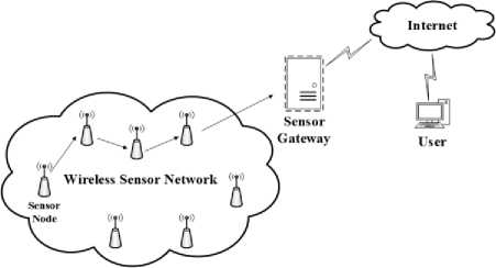
Fig.1. Wireless Sensor Network

• B.    Cloud Computing

Cloud computing, also on-demand computing, is a type of internet based computing that provides an on-demand service access through shared processing resources [14]. The term cloud in cloud computing is used as a metaphor for ‘ the internet ’. As a result, all of the cloud services (e.g. software, platform, infrastructure etc.) are delivered to the user through the internet.

Cloud computing can be thought as a model of network computing where the servers can be in the form of virtual machines or physical machines in the cloud. To achieve coherence, it relies on the resources to be shared through different cloud services [15].

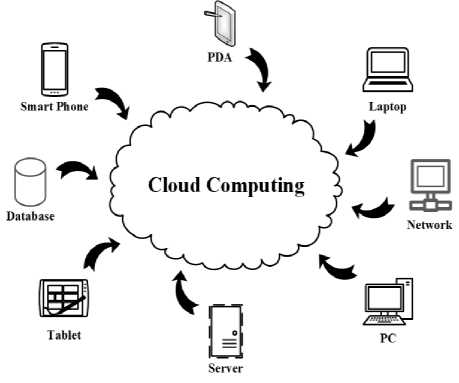
Fig.2. Cloud Computing

Cloud computing also provides great and convenient user experience because the end users don’t need to think about the actual location of the servers. They can have the service by simply connecting to the server using a login panel [6].

• C.    Integration of WSN and Cloud Computing

In sensor-cloud infrastructure, the WSN is integrated with cloud environment in order to achieve convenient processing and storage. This approach allows the sensor network to accumulate and transmit all sensor data to cloud in a periodic time interval.

The sensor-cloud infrastructure (i.e. the integrated infrastructure of WSN and cloud computing) is a unique sensor data storage, analyzing and monitoring platform that uses scalable cloud computing approach to providing excellent data analysis and visualization [16].

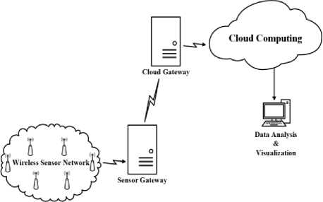
Fig.3. Sensor-Cloud infrastructure

In this approach, the limitations of WSN such as limited storage, processing, and power consumption are overcome. As cloud computing has massive storage and processing capability, it enables the sensor network to collect the huge amount of data by connecting it to the cloud through gateways. The sensor gateway collects the sensor network data and after compression, it sends the data to cloud gateway through the internet.

• III.    Similarity-Based Classification and Compression

• A.    Similarity and Distance

The purpose of similarity and distance measure is to compare two sets of data (record, vector) and calculate a single value that represents their similarity. These measures are essential to understand the closeness property of two data sets. But choosing an appropriate similarity measure is also important for classification. There are several ways to measure the distance for a different pattern of data sets in classification and clustering. Some of them are as follows:

• 1)    Euclidean Distance:

Euclidean distance [17] is a special case of Minkowski distance. It is the (straight line) distance between two points in two-dimensional space [18]. In Cartesian coordinates,      if       X =( ^1 , %2,…,x_n )      and

Y=(У1 , y2,…,Уп ) are two points, then the distance (d) from X to Y or from Y to X is, d = √(%1 - У1 )2+( ^2 - y2 ) 5 +⋯+(%„ - Уп )2

=√∑ "=1( ^xi ^- Vi )²                            (1)

angle between them. It evaluates the judgement of orientation rather magnitude (i.e. the cosine similarity of two vectors with the same orientation is 1, if the angle between them is 90° then the similarity is 0, and whether the vectors are diametrically opposite of each other then the similarity is -1, independent of their magnitude [20]). Cosine similarity is specially used in non-negative space and the outcome lies within [0,1]. Given two vectors of attributes, p and Q , the conise similarity, cos (9 ) , is represented using a dot product and magnitude as p.Q        ∑ ^PiQi similarity = cos(9)=    .    =

‖^p‖‖ Q _‖= _√∑ i=l Pl √∑ ^iQt

• B.    Classification using Machine Learning

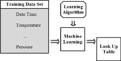
In statistics, the classification being a supervised learning approach is one of the procedures of classifying a new set of records to which of a predefined class it belongs on the basis of a training data set with known category membership. Here the predefined classes can be identified by various methods such as machine learning.

Machine learning is a method used to build complex models that can give predictions where a training set of correctly defined observations is available [21].

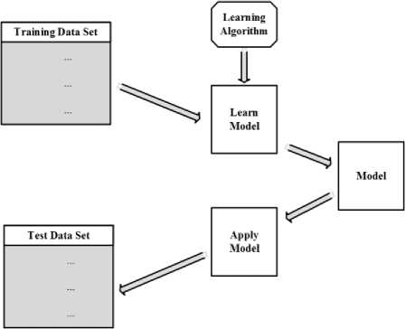
Fig.4. Classification using machine learning

These analytical models can help us to produce reliable inferences and hidden insights from the trends in the data [22].

• C.    Lossless Compression

Lossless compression is a type of data compression that allows the compressed data to be decompressed in a manner that will not have any data loss [23].

• 1)    DEFLATE Algorithm:

Deflate [24] is an efficient lossless data compression algorithm that compresses data using a combination of the LZ77 [25, 26] algorithm and Huffman coding [27]. Several free and open source data compression applications (e.g. 7-Zip [28]) uses Deflate algorithm. The use of Deflate algorithm is also found in some popular file formats such as ZIP, gzip, PNG, PDF and so on.

• IV.    Problem Description

The communication between WSN and sensor gateway can be done by means of Bluetooth or wi-fi. On the other hand, the communication between cloud gateway and cloud environment can be of wired or wireless.

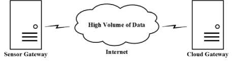
Fig.5. Target area of optimization

The most difficult part is the communication between sensor gateway and cloud gateway where a large-scale data is to be sent frequently. Since the internet is considered to be the communication medium, it requires a very high amount of bandwidth leading heavy transmission, high internet cost and lack of data security.

• V.    Proposed Framework

As we know that sensor networks generally sense data in a periodic time interval, we can expect a lot of similarities in the same time period of the different cycle (a complete period of time) because the data generally follow seasonality.

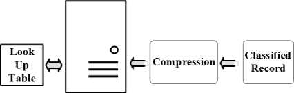
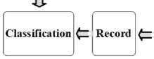
In our proposed solution, instead of sending similar records (a set of sensor values in a specific time interval) again and again we prefer to send a single code which will represent the entire record and before sending it we are also using a compression algorithm (deflate algorithm [24]) which will reduce overall bandwidth requirement. The workflow of the proposed framework is depicted in Fig. 6.

Cloud

Gateway

Fig.6. Flow diagram of proposed framework

Sensor

Gateway

First of all, we need a Look_Up_Table (a list of predefined records with individual codes) which will be used to measure the similarity. The Look_Up_Table can be built by mining (using machine learning approach) the prior data for a complete cycle.

At this point, the Look_Up_Table has to be available at both gateways (sending and receiving). For a new record, it should be compared with each record of the Look_Up_Table. If a standard amount of similarity is found, the corresponding code is sent instead of the total record. The dissimilar records will be added in the Look_Up_Table and after each cycle, the Look_Up_Table is to be updated based on the frequency of hit ratio.

• VI.    Implementation

In our research, we have considered environmental data consisting of six sensors (Air Temperature, Dew

Point, Humidity, Pressure, Wind Speed, Sea Level Pressure) which are collected at one-minute interval [29]. We have obtained more than 5 lac records from the data source [29] for the one-year time frame.

• A.    Time Series Analysis in order to find Seasonality

As the data is collected at fixed time interval, we are considering it as a time series data which must have seasonal and cyclical effects. Here we are taking a single day as a cycle and each hour is considered as a season. As a result, there will be twenty-four seasons in a single cycle. For each month, we have calculated the seasonality to separate the overall seasonal effect of a year (complete cycle).

1) Stationarity Test:

First of all, we have identified the stationarity of the data using Dickey-Fuller (ADF) test.

Test interpretation:

Hq : There is a unit root.

Hq : There is no unit root. The data is stationary.

Table 1. Stationary Test

Parameter	Value
Tau (Observed value)	-4.0525
Tau (Critical value)	-0.9079
p-value (one-tailed)	0.0070
Alpha	0.05

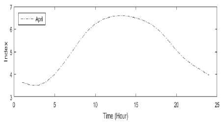
Fig.10. Seasonal index (April)

As the computed p-value is lower than the significance level alpha=0.05, we should reject the null hypothesis Hq , and accept the alternative hypothesis H_a . The risk to reject the null hypothesis ^o while it is true is lower than 0.70%.

2) Seasonality Measure:

For a whole year we have considered each day as a cycle and each hour as a season, so we have measured the seasonal effect for each consecutive month as well as the complete cycle (a year).

We have calculated the seasonal indices for twenty-four seasons of every month which will explain the seasonal effect within them.

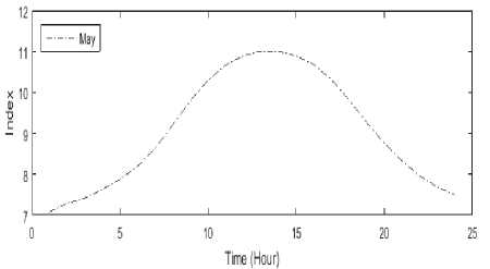
Fig.11. Seasonal index (May)

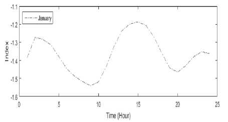
Fig.7. Seasonal index (January)

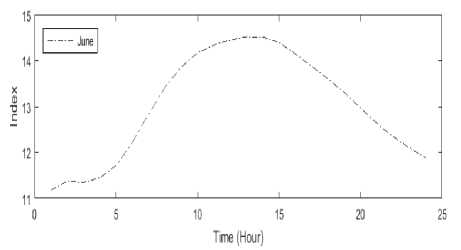
Fig.12. Seasonal index (June)

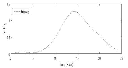
Fig.8. Seasonal index (February)

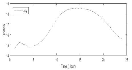
Fig.13. Seasonal index (July)

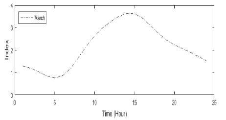
Fig.9. Seasonal index (March)

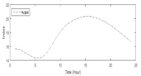
Fig.14. Seasonal index (August)

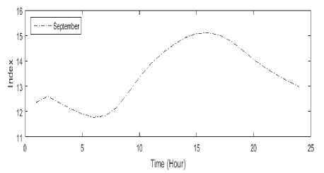
Fig.15. Seasonal index (September)

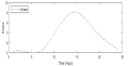
Fig.16. Seasonal index (October)

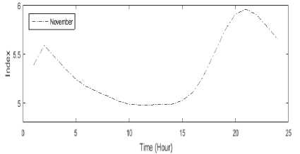
Fig.17. Seasonal index (November)

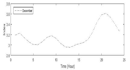
Fig.18. Seasonal index (December)

From Fig. 7-18, we can notice an existence of the almost similar pattern from February to October where the graph of seasonal indices follows a route from low to the zenith and resting at low again. For November to January, there exists another pattern having multiple ups and downs. Now we can conclude that there exists seasonality within successive months.

Since our main concern is to find similarity among each record in the data, so we have also identified the similarities between the successive months.

According to the fig. 19, we can see that there exist similar seasonal indices in between two halves of the year. As a result, we can expect that in spite of having similarity within each month there will also exist similarity among rest of them.

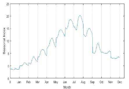
Fig.19. Overall seasonal index (Total Year)

• B.    Generating the Look_Up_Table

Since we have found seasonality at the previous step so it is obvious that there will be a lot of similarities in between successive seasons. For this reason, the Look_Up_Table has been generated using machine learning approach.

• C.    Similarity Measure

For each record, we have considered that to be a Look_Up_Table record if the Euclidean distance of it with every other record is less than a specific threshold, k.

Here, k is the maximum allowed Euclidean distance which is determined by combining the standard deviations for all variables.

_∑ Si ( Hi -1) ^S1 =_∑  ( nt -1)

к    ( П1 -1) $i +( ⁿ2 -1) s| +⋯+( П1 -1) S

J       ⁿl + n₂ +⋯+n_m - m

Using equation (3) we found к ≈4.6 and we have got 1585 records in the Look_Up_Table which have classified about 98% of total data with a good hit ratio.

For each record, we have calculated the Euclidean distance with every other record. If the minimum distance is less than к (threshold value) then we have considered the record as a new entry in the Look_Up_Table .

• D.    Classification of new data

At this step, we have got the Look_Up_Table for a complete cycle which will be used in order to classify new records. Now for the next cycle, when a new record appears, it has been compared with every Look_Up_Table records. If similarity (using previous similarity measure) is found, then only the corresponding code has been sent to cloud gateway and the frequency has been updated for that particular record. Otherwise, the raw record has been sent to the cloud gateway without any modification and considered as a new

Look_Up_Table record.

After a complete cycle, we have an updated Look_Up_Table with different hit ratios. For the next complete cycle, we have eliminated the least used records from the table.

• VII.    Result and Discussion

To measure the performance of the proposed framework, we have done the required simulations for different scenarios and the outcomes were also compared with the traditional approach and [5].

• A.    Overall Bandwidth Comparison

The primary concern of our research was to find the possibility of bandwidth reduction among sensor-cloud communication. For this reason, we have calculated the required bandwidth for every single transmission and found a significant difference between traditional and proposed approach. We have also compared the cumulative bandwidth for both cases (with and without compression) as well as with the traditional approach.

From fig. 20, we can see that a remarkable amount of bandwidth is being reduced by using our proposed framework.

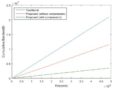
Fig.20. Cumulative Bandwidth Comparison

Though we have considered a limited number of sensors (i.e. six in our case), the result will be more noticeable when the network expands.

• B.    Overall Time Comparison

The time in which a transmission completes is very important in almost any type of communication. For this reason, a framework can be considered efficient if it reduces the bandwidth consumption and takes an acceptable amount of time for processing.

In our research, we have considered 128 Kbps connection between the sensor and cloud gateway.

Here, 128 Kbps ≈

≈ 32 kBps

≈ 32 × 1024 bytes / sec

≈ 32768 bytes / sec              (4)

According to equation 4, we can say for any X bytes we will need X /32768 sec or 0.31 X millisecond. So it is clear that when the bandwidth increases the sending time also increases. For our proposed framework, we have measured the processing and sending time for every single record. The following graph describes the cumulative time comparison between the traditional and proposed approach.

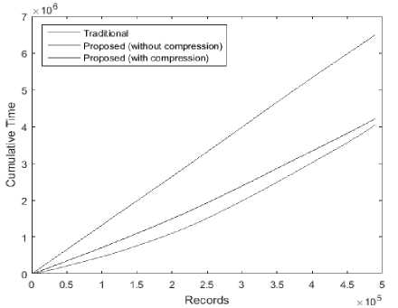
Fig.21. Cumulative Time (Processing and Sending) Comparison

According to fig. 21, we can see the time that our proposed framework (without compression) takes to process and send the data is less than the traditional approach. The graph also explains that the required time even after compression is less than the traditional approach and the difference between with and without compression is very minimal.

• C.    Residual Measure

After applying the framework, we have also compared the received data for both traditional and proposed approach in order to measure the changes.

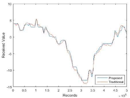
Fig.22. Residual Measure of Received Data

From fig. 22, we can see both lines are following the almost same path and the difference between them is negligible.

• D.    Performance Comparison

To compare with the result of [5], we have additionally calculated the required bandwidth for the first 15000 bytes using proposed framework with and without compression.

Table 2. Results of [5]

Scenarios	Size in bytes
Before compression	15000
After compression (without using neural networks)	980
After compression (with using neural networks)	400

Table 3. Results of Proposed Framework

Scenarios	Size in bytes
Before classification and compression	15000
After classification (without using compression)	1021
After classification (with using compression)	85

In our proposed framework, the bandwidth consumption without using compression is a bit higher than the framework proposed in [5]. But after using the compression algorithm, we have got a significant amount of bandwidth reduction and the data misclassification error is minor.

• VIII.    Conclusion

The combination of sensor-cloud is becoming very popular in recent years as it provides a new framework of accelerating service innovation and cross-disciplinary applications that span organizational boundaries. In sensor-cloud architecture, the communication between WSN and cloud computing is a challenging task as the required bandwidth is very high.

Our proposed framework can minimize the robust bandwidth requirement of sensor-cloud communication where the amount of data loss will be negligible and the required time for the transaction is also reduced to some extent. From our research, we have found that our proposed framework is providing 4.7 times better performance compared to related research.

We will continue to extend our research to observe the proposed framework in different real world application to optimize the overall performance.

Acknowledgment

We would like to express our gratitude to Heikki Junninen, Antti Lauri, Petri Keronen, Pasi Aalto, Veijo Hiltunen, Pertti Hari and Markku Kulmala for the data source although any errors are our own and should not denigrate the reputations of these persons.