Effort estimation of back-end part of software using chaotically modified genetic algorithm

Published Online January 2019 in MECS

The process of estimating the amount of effort which is expressed in final cost or person-hours for developing a software project is termed as Software development effort estimation. The inputs which are taken for this prediction process are budgets, project plans, analysis of investment, bidding rounds and plans of iterations [1, 2, 3]. From the last few decades, the process for developing software for various software related project has advanced through heterogeneous stages. Software project’s requirements and types have also got completely advanced. The process of developing software is getting more and more complex day by day because nowadays the software projects are bigger in size and more complex unlike in the past where they were simple and less amount of requirements were also less in size [4, 5, 6]. Due to the increment of the size of the software projects, the developing cost has also increased parallel. While the back-end part of the software was being neglected a few years back because the contribution of the back-end part was quite negligible. But in today’s scenario, the backend part of a data-intensive application plays a vital role during the effort estimation of the software development due to its exponential growth [7].

Since the availability of research work on SDEE of back-end part of the software is quite less, therefore it is completely a new field in which more research can be done. Many of the earlier complete research work mainly focused on the SDEE of the back-end part of the software in terms of the size of the ER (Entity Relationships) diagram and the complexity [7].

The size of the back-end part of the software, their schedule a cost and also the role of the defect are hugely affected by the ER model’s complexity. The overall required effort estimation gets increased if there is an increment in the complexity of the ER model [8]. The main focus of previously done researches was on the relationships among the entities, count of the entities and the attribute’s count. These were the components that were recognized as being the main factors while determining the complexity of the structure of an ER diagram [7, 8].

Moreover, for precisely estimating the size and complexity of the database of the software some more factors can be taken into consideration which may be available in the EER (extended ER) or ER like aggregation knowledge and its extensions, specialization/ generalization design constraints, relationship’s degree, referential integrity constraints death, entity sets relationships which include mapping cardinality and specialty of attributes present in entity set [5, 7, 8].

For the problem of SDEE, this paper has proposed an evolutionary learning algorithm. The proposed approach has been tested over two datasets. One of them is existing and the other one is a self-developed dataset. The proposed model’s robustness and its performance were tested by three well-known performance metrics which are illustrated further in this paper.

Further, this paper is divided into ten subsections including the introduction part. Section-II presents the overview of back-end estimation along with the related works found in the literature. Section-III contains the basic methodologies used for the proposed technique. Section-IV presents background knowledge on MNN. Section-V describes the proposed evolutionary process. Section-VI describes the genetic operations. Section-VII contains the knowledge about performance measures. Section-VIII describes the simulation and experimental analysis. Section-IX presents the conclusion of the proposed work along with future scope which is described in section-X.

• II.    Related Works

Since the growth of the software projects, the back-end part of such projects also increasing exponentially. This is making it be a pivotal contributor to the overall effort of the software projects. Following are some of the related works that have been carried out in this particular field.

The proposition of four effort metrics for the database or back-end part of the software which can be derived in accordance with the complexity level of the ER diagram has been carried out by Samaresh Mishra et. Al .[7]. The proposed work includes a new model for estimating the complexity of the database and also the size of the database. The experimental analysis has shown that the total effort which is required to create a database is directly proportional to the database’s complexity. Bushra Jamal et. al. [9] have proposed an empirical validation of relational database metrics which is being used for estimating the effort of the back-end part of a software project. The proposed model is used for estimating the effort as well as some database objects because of its flexibility. The results that are found in this paper have been analyzed with an actual effort which is necessary for developing a database and found its prediction is more precise. With the help of an ER diagram, a model for estimating the effort has been proposed by Samaresh Mishra et. al. [8]. The model takes the complexity of the ER diagram of the back-end part of the software for estimating the effort. The metrics used in the model include relational size, the size of the entity and the size of semantic integrity constraints. COCOMO model is used for calculating the total required effort. The results show that the accuracy of the prediction has increased up to 4% from 3%. Parida et. al. [10] analyzed models that are usually used for the estimation of the size of the backend part and for the effort estimation. Along with the front end development, development of the back-end also plays a pivotal role. The two components which are responsible for the cost of the back-end part are the size of each and every data item and the structural size of the database. The experimental results have shown how the effort estimation is carried out for the back-end part by using ER diagram’s artifacts and it also shows how to increase the productivity for the calculation of the backend part’s actual effort, of any business software. Samaresh Mishra et. al.[11] identified that for effort estimation required for the development of the database is directly proportional to the size of the relational database model and intricacies. The verification of the model has been carried out on small size projects completed by the students. The experimental analysis is done using DCS (Database Complexity and Size) where the main focus is on data. A detailed study was carried out by the software’s requirements for coming to this conclusion. Functional, document and data are the three components that are allowed by the software products. Database’s volume is the main factor for the effort which is needed for the database development. A bunch of verified models for the prediction of the database’s size by utilizing ER and EER (Enhanced ER) diagram has been proposed.

• III.    Methodologies Used

• A.   Database size estimation based on ER-diagram

(DSEBER)

The database plays a pivotal role in implementing the data-intensive software. Since the relational database management system (RDBMS) is capable of specifying many integrity constraints related to business, it is utilized for developing the back-end of the data-intensive software products. Therefore, for developing and designing a database it becomes necessary to focus on the ER Modelling approach since object-oriented methods or functions are used by RDBMS for the back-end part [7, 8, 12]. The factors which are responsible for the effort for developing a database is the relationship complexity between the data items, database size and data item numbers. Below is Lifecycle of database development:

• •    Conceptual or ER modeling

• •    Logical modeling

• •    Physical modeling or process of implementing

Refining of the above life cycle process of database development is done because the estimation becomes more precise with the flow of the process. For the estimation of the size, the conceptual modeling phase has been considered better phase by utilizing artifacts of the ER diagram in this suggested work [7, 8].

• B.    DSEBER Metric

A proposed metric is used for measuring the total relationship, entity, and size of semantic integrity constraints from the ER model’s artifacts. For the measurement of the size of the database from the ER diagrams, the given factors are being considered [7, 8].

• a.    Total Entity Size Estimation (TESE)

The factors that are responsible for the size of the structure of the entity are associations between the entity sets, its generalization/specialization hierarchy role, and a number of entity sets. Following factors are considered for the prediction of the size of an entity [7, 8]:

• •    Count of similar attributes (COSA)

• •    Count of derived attributes (CODA) where values can be derived from the result of calculation with the generated lines of code when the

implementation is being carried out.

• •    Count of multivalued attributes (COMA) which results in the creation of an additional table.

• •    Count of many to one or one to one participation (COM1P) which exists among various sets of entities.

• •    The depth of inheritance (DI)

Entity size can be measured with the help of the factors described in Table 1 [7, 8].

Table 1. Factors Considered For Entity Size

Factors	Description
COSA	Similar attribute’s count
CODA	Derived attribute’s count
COMA	Multivalued attribute’s count
COM1P	Many-to-one or one-to-one participation’s count from one entity set to another entity set
DI	Inheritance depth of the entity

The vital task of COM1P is to establish a referential integrity constraint and the increment in attribute’s count on the entity set by utilizing foreign keys. The relation between the foreign key and COM1P is that both are directly proportional to each other. For the indication of the count of primary key with a numeric figure, DI is used for representing them. (COMA + 1) numbers of relations are being produced by COMA for keeping the relations under 1NF [1]. By adding the simple count of the primary and foreign key which are inherited in generalization, multivalued attributes, the calculation of count of attributes can be done [7, 8]:

COA = COM1P + CODA + DI + COSA + COMA (1)

If the size of the primary key of an entity set is denoted by Size pk , where attribute’s count is denoted asSize_pk = 1, where the primary key is derived from a single attribute andSize_pk = n, when a composite primary key which consists n number of attributes [7].

When there are many multivalued attributes present in the entity set and maintenance of the relation should be in 1NF, then the base relation is being decomposed into (COMA+1) count of relation.

Determination of the count of an attribute can be done by (count of attributes in base relation (COA)-COMA) and derived relation’s size from the base relation can be calculated by adding the base relation’s primary key and the multivalued attributes. Now the equation by which we calculate the size of derived relation is giver below as [7].

SizeDR = (SizepK) + (SizeMA ) (2)

Here, the size of the derived attributes is represented by SizeDR and SizeMA is the notation for the multivalued attributes. When multivalued attributes consist of a single-valued attribute then, SizeMA =1 and when multivalued attributes consist of n number of attributes then, SizeMA = n. Entity set’s size can be determined by adding all the attributes of the relations which are produced from the entity sets, as given [7, 8]:

SizeEs = (SizeBR) + ^’^(SizepR);    (3)

Where entity size is denoted bySize_ES , base relation size is denoted by Size_BR and derived relation size is denoted by Size_DR . Here, the COMA and the number of derived relations are equal, which have been derived while maintaining the 1NF property from the relation.

Calculation of ER diagram’s total entity size which is denoted by TotalES can be represent as [7]:

Total Es = Z yIi (Size Es ) y              (4)

The number of total entity sets present in the ERD is denoted by CE.

• b.    Total Relationship Size Estimation (TRSE)

The factors which are responsible for relationship set’s structural size are a count of entity set which is associated and count of the descriptive attribute. Each many-to-many relationship results in generating a new relation. The factors mentioned above are given in Table 2. [7, 8]:

Table 2. Factors Considered For Relationship Size

Factors	Description
NODA	Number of descriptive attributes
DMMR	The degree of many to many relationships
AGG	Count of aggregation

The size of relationship set can be found by adding a count of foreign keys that are present in it and descriptive attribute which relies on the count of aggregation that takes part in this relationship and the count of the entity. They can be represented as [7]:

SizeRS = NODA +2 x (SizePK), if DMMR = 1 (5)

Size_RS = NODA + S f₌T^R (Size p_K ) i , if DMMR > (6)

Size of relationship set is shown by SizeRS and entity set count is shown by i, which is associated with this relationship set.

For DMMR = landDMMR = 2, foreign keys count is unchanged.

Sum of the size of all the relationship in Eq. (7) is used to get the total relationship set contained in this category [7]:

^TotalRS = E k=i^(SizeRs^{) (7)}

Count of a many-to-many relationship is shown by CR and the total size of the relationship set is shown byTotalRS [7, 8].

• c.    Total Semantic Integrity Constraint Size (TSICS)

A few business constraints are found in the early development stage in form of semantic integrity which is caught while ER modeling. For performing these type of constraints, procedural language is used. So the evaluation of the size of such semantic constraints is done on the foundation of LOC which are required for performing. Thus, the overall size of all semantic integrity constraints is given in the Eq. (8) [7]:

Totalsc = ^^=1(LOC)k            (8)

Here TotalSC shows the whole size of semantic integrity constraints and j shows the whole count of the semantic integrity constraints.

• d.    Total Database Size from ER Diagram (TDSERD)

By taking into account the count of entity set, attribute required for entity set and relationship, relationship set count with the mapping cardinality, the database size can be evaluated from the conceptual design stage and it is also reliant on structural complexity rooted in the depth of the inheritance o entity set within the hierarchy of specialization/generalization and linked count of aggregation. Eq. (9) shows the total database size acquired by ERD [7, 11].

Total ERD = Total Es + Total Rs + Total cs     (9)

where Total ERD shows the total size of the ERD.

• C.    DSEBER Process model

In Fig. 1, the portrait of the DSEBER model’s diagram is given. It is used for predicting the effort required for developing the database with the help of measured suits of DSEBER over the phase of conceptual modeling of development of the database [7, 8, 9]. By measuring the size of the database with the help of the proposed DSEBER’s cost metrics, the effort which is required for developing the database can be estimated. The requirements gathering and the requirements analyzing process are done at the early stage methodically, as per the model’s need. The construction of the ER diagram and extended ER are carried out to capture the requirement of data as a factor of the analysis model. After that, the calculation of the total size of the database is done by using the proposed DSEBER cost metrics. Finally, by using the total size of the database which was calculated earlier, the effort which is required for developing the database is predicted with the help of the COCOMO model. In our proposed model we have used DEP (CMGA) model for predicting the effort required for building a database which is further discussed in the paper. Various objects which were unknown, during the early stages of the development of the database, showed out during the phase of implementation [7]. Cardinality’s degree and mapping, relationship (based on number and type of attributes that are present in it), generalization and specialization and entities are those components which are used for the database’s size estimation. Therefore the DSEBER model which is proposed here may play a vital role in the conceptual phase of the database system of any software [7, 8, 11].

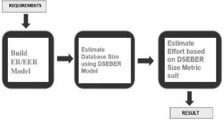
Fig.1. DSEBER Process Model

• IV.    Background on Mnn

Morphological Neural Network (MNN) can be described as artificial neural networks (ANNs), which carry out the basic transaction from the mathematical morphology (MM) between entire lattices at each and every network processing unit (NPU). Here we basically focus on the definition of MNNs by the algebra of lattices [13, 14].

If each and every finite and non-empty subset of Chas a supremum and infimum in C, then C (a partially ordered set) is said to be a lattice. For any X c C, the symbol Л X is used for representing the infimum [14].

For any index P, ЛХ can be represented as K_pEPx^p , when X = [x^p,p E P}. Also, supremum o f X (V X) can be described by using same notations [1the 0, 11].

Let C and D be two lattices. Then a mapping such as V: C ^ D is termed as increasing if and only if Vx,y E C, the following statement is satisfied [14, 15]:

x < y ^ V (x) < V (y)           (10)

By considering C as lattices, then a partial order on Cn can be described by setting [15]:

The outcome of C ” (partially ordered set) derived from Eq. (11) is also termed as a lattice. It is also called as product lattice [14, 15, 16].

This is very important to take into account that the lattice C is said to be complete only when each and every nonempty subset comprises a supremum and an infimum in C. The product lattice Cn is complete only if the completeness of C lattice is achieved [14, 16, 17].

Decomposition of mappings between the complete lattices in terms of fundamental morphological operators is one of the major issues.

Let δ and ε be two operators from C to D, where both C and D are complete lattices (CLs). Then according to Banon and Barrera’s decomposition theorem:

Theorem: V: C ^ D, which is the increasing mapping, between C and D,where both C and D are complete lattices can be constructed as infimum of dilation or supremum of erosions.. For index P and Q, the existence of dilation 6P and erosion eq can be defined as [18]:

• V    = ^ _£^q = ^6^p pep     qeQ

The decomposition theorem by Banon and Barrera has worked as the foundation of many MNN model’s learning algorithms. The basic morphological operators in the models which occur during the decomposition process are believed to follow a special form where an extra structure of algebra is required along with the CL structure.

The main focus of this paper is on №_±ю (complete lattice), because the problem of SDEE can be structured in terms of function K ” _ro ^ №_±ю. (where the count of so the software project’s variable is represented by n).

Let E e R^{u x w} and F e R^{w x y} be two given matrix. Then the max-product of E and F matrixes can be represented as [14, 18]:

G = E IV](13)

Similarly, the min-product of the above to matrixes can be computed as:

H = E IV] F(14)

These are described in the given Eq. (15) [15]:

gpq = A^1(epk+fkq) = V^(epk+fkq)(15)

Let us take up some operators ee, SE:R±m ^ R±M for E e R“ x vthen [14, 15, 18]:               ""

Ee(x) = ET A X(16)

5E(x) = ET V X(17)

Where T represents the term transposition of given set. Algebraic erosion is denoted by e_E and algebraic dilation is denoted by 6_E from CL R ^ _TO to R^ , This Eq. (12) suggests that mapping function V: R “ ^ R, which is an increasing function and can be estimated as [15, 17]:

• V - Д6 P V pep

or v - y£q qeQ

Wherer^p and s^q e K “ are the vectors for some finite indexP and Q .

In case of P = 1 and Q = 1, the vectors r,se K“ can be used for the approximation of the mapping function V: Ru ^ R and can be represented as [14, 15, 17]:

V -5_T                 (20)

Or

V - -                    (21)

• V.    The Process of Evolutionary Learning

One thing that should be noted down is that the variables like a, b and Л needs to be tuned for the DEP model. Therefore, the factor of weight which is going to be used for the training’s process is mentioned in Eq. (18) [14, 19, 20].

W = (a,b,K)              (22)

Until the CMGA iteration’s convergence is found out, adjustments are being carried out with respect to the criteria defined for error. The representation of chromosomes weight vector of j^th individual from g^tk generation is done byw ^ ⁸ ) . For determining the fitness function which is denoted byff(w⁽⁸⁾), the weight vector must be altered. This should show the quality of solution which is achieved by configuring the variable on the system. Fitness function is determined as given in the Eq. (23).

fKw^) = Л/ . e ' lk;             (23)

The number of input patterns is represented by N and the error (instantaneous error (IE)) is represented by e(k) and can be computed as [14, 20]:

e(k) = d(/)- y(k)              (24)

Here, the desired outcome signal is denoted by d(k) and obtained output is denoted by y(k) which is for a training sample that is represented by k.

For parameters adjustment of DEP model and predicting values of the model, the below-mentioned stages are followed in DEP (CMGA) process.

• A.    Initialization of Population using Chaotic Opposition based Learning Method (IPCOLM)

Initial population values always affect the convergence speed and the likely predicted output of the evolutionary algorithms. A better convergence speed can save the iterations of algorithms from getting trapped in local optima problem. Hence, instead of using a random initialization of the population using chaotic opposition based learning method also represented as IPCOLM has been used for gathering more likable output. The sensitivity and randomness are directly dependent on conditions defined initially by chaotic maps. These maps can be utilized to initialize the initial population for increasing the population diversity through extraction of search space information. After using this approach, the CMGA algorithm’s convergence speed also gets increased. For this approach, the sinusoidal iterator has been used which is given in the Eq. (25) [22].

Sch_i+1 = sin('n:Sch_i),Sch_i E [0,1],i = 0,1.. i_max  (25)

Here, i denotes the count of iterations and i_max denotes the maximum possible chaotic iterations. The steps for IPCOLM can be referred from Algorithm 1. (referred as Fig. to 2).

Algorithm 1: Steps for IPCOLM Algorithm begin

(IPCOLM) [22]

Data: Initialize maximum chaotic iterations as i_mal = 300

Pop,1IC = P

Result: Рормы for j=l to U do for k=l to V do

Initialize randomly variable Schok hi the range: a,be[-l,l] and Ae[0,1];

for q=l to imax do

| Schqk = sm(,~Schq_vk')

end

Zjk ⁼ ^min_k + Schqk\ZmaTk ^— ^mfnt)

end end

(—Run Opposition Based Learning Method—);

for j=l to U do for k=l to И do

| OPZpjk — Zmink *i" Zmazk Zkj end end

Perform the selection of U fittest individuals from the population set (2((/) UOPZ(U') and set them as Popi_nili_ai;

end

Fig.2. Steps for IPCOLM Algorithm

The process of CMGA starts a loop which consists of the stages for an objective which is minimizing the fitness function ff:^⁷¹ —> R . This is defined in the Eq. (23). The dimensionality defined for weight vector of the DEP model is denoted by h and it can be computed as 2h+1. The loop consists of the process of selection followed by the genetic operators such as crossover and section. The crossover operator and mutation operator is applied on a pair of the parent of chromosomes opted from the selection process for further reproduction of new offsprings. Primary focus here is to select the best individual from the given population. Let the value of Pop_s i _ze = 10 [14, 21, 22, 23, 24].

• B.    Process of Selection

For going through the genetic operations, two numbers of chromosomes are selected from the population. For reproduction of new off-springs. For this spinning, the roulette wheel technique has been applied. Better child chromosomes are said to be produced by the parents with high potential. The chromosomes which will have a better fitness value would have more chance of getting selected. The selection method of the chromosome C j , can be executed by using the probability P j . Follow the given Eq. (26) [20, 23].

ff(C j )

^Pj = yPoVslze   _r ,^{,j   1,2,}^^., ^POpslze         ⁽²⁶⁾

^ k=i    JJ ^(c k )

Cumulative probability CP j of the chromosomes C j is determined in the Eq. (27).

CP ) = lL 1 CP_k,j = 1,2.....P^P size      (27)

The process of selection starts by generating a random numberd E |0,1| which is a non-zero number (floating point). The chromosome C_ionly selected, if and only if the following condition given in Eq. (28) is satisfied:

CP_j-1j-1, (CP₀ = 0)          (28)

The observation that is done through this process of selection is that, the chromosomes which have a greater ff(C j ) will possess a greater opportunity for getting chosen. Therefore the best chromosomes among all the other chromosomes will generate number of offspring and the average would live while the worst ones will die. The genetic operations only undergoes in the selection process on two chromosomes only, which are chosen.

• VI.    Genetic Operations

New off-springs are created by applying the genetic operation (operator) on the selected parent chromosomes. The genetic operation consists of a process of crossover and mutation process which are described below:

• A.    Process of Crossover

The crossover operation is utilized for helping in the exchange of information between the two selected parents (Vectors W®, W_b^g) E K, where a and b are indices in the range [1, P]), with the help of the roulette wheel approach. For the recombining process, the crossover operators are utilized, which help in the reproduction of four new child chromosomes or offspring ( of f s₁, of f s₂, of f s₃, of f s₄ ER " ) which is mentioned in the Eq. (29), (30), (31) & (32) given as follows [14, 20]:

of f s₁ = W g +W b

off 8 2 = max (w_a^(g),W_b^(g)) u + (1 - u)w_max   (30)

offs₃ =min(w_a^(g),W_b^(g))u + (1-u)w_m i„     (31)

offs₄ =

■ (^ o⁰) * W ⁽⁰⁾' ⁾ + ^(1—'ll⁾⁽ Wmax ^+w min ⁾

The vectors min( W ag) , W^(g) ) and max( W ag) , W^(g) ) are used for denoting the minimum and maximum of individual respectively. The crossover weight is given byu E [0,1]. Here the value ofu is 0.9 (Closer value to 1 represents the direct contribution of parents to the reproduction process using crossover). The representation of the vectors having min and the max possibility of the values of the gene are done by W_m [ _n & w_max respectively [14, 20].

After the conclusion of the crossover, process produce, the fitness of each newly generated off-spring is calculated and off-spring having best fitness value (i.e.

least value) will be selected as best of all. The representation of the resultant best crossover off-spring is done by the vector of f s_best E K ” , which then performs the replacement process by replacing the individual which comprises the worse fitness in the given population (i.e. W^ se with the worse E [1,P] [14, 20].

• B.    Process of Mutation

Let set the Prob_Mut = 0.1 as probabithe lity of mutation. Thenmo₁,mo₂,mo₃, E K are the three new mutated offspring that are created by usingoff s_best and can be computed as [14, 20]:

mof f j = offs_bes t + t j V j ,   j = 1,2,3       (33)

Vector t [ satisfies the inequalities W_m [ _n <  of f s_best + t [ <  W_mnx , where i=1, 2, 3. The range of vector v is chosen among[0,1]. It also satisfies following condition: vector v₁ comprise only one non-zero chosen entry (selected randomly), v₂ has a randomly selected binary non-zero entry and v₃has constant vector value 1. After the production of a a newly mutated off-springs, again the fitness of all three has been calculated and then for association of them withthe in the population fothe the llowing scheme has been takenwith the help of a randomly generating numbers (Rand) from the range of [0,1] : If Rand <  Prob_Mut then the replacement of W worse within population range i.e. [1, P] is done with the mutated offspring having least fitness value, else the mentioned steps are being followed for j = 1,2,3 :

W wors _e if the fitness value of the mo j < W vor _se then the mo j will replace the W^se in order to form the new population [14, 20].

Moreover, the stopping criteria used for the proposed DEP (CMGA) process is given as: (i). CMGA_qen = 10000 which is the number of maximum generation (ii). TEP < 10^-6 which is training error process of fitness function.

The steps of DEP (CMGA) process is given in Algorithm 2. (can be referred to as Fig. 3):

Algorithm 2 : Steps for DEP(CMGA) Algorithm

DEP(CMGA)[14, 20]

Data: Pop_injh„i supplied from the IPCOLM algorithm

Result: Predicted Value

Perform initialization of CMGA parameters according to [19]:

Perform initialization of stopping criteria;

£-0;

while Termination criteria is not satisfied do

' g-g+i;

for j=i to P do

Perform initialization of DEP parameters by considering values from w^ ;

Estimate the value of у and IE for all given input patterns;

Calculate the fitness ffi,w^^ of each individual using eq. 23;

end

Perform the selection process Xr select two fittest paranets (itv and a1^*) from the current population for j=l to .{ do

Perform initialization of DEP parameters by considering values from of fsj\

Estimate the value of у and IE for all given input patterns;

Calculate the fitness ff(offsj) of each individual using eq. 23;

end

°ff^sU-«< denotes the best evaluated offspring;

for j=l to 3 do

Perform initialization of DEP parameters by considering values from moffa

Estimate the value of у and IE for all given input patterns;

Calculate the fitness f f{mof fj) of each individual using eq. 23;

end of fsbc»< will replace Ulj if Hand < ProbMut then

| then moff, will replace а-йгм end end end end curl

Fig.3. Steps for DEP (CMGA) Algorithm

• VII. Performance Measures

For the performance evaluation of the proposed system after successfully implementing the idea, this paper has used three popular measures of performance (i.e. mean magnitude of relative error, prediction and evaluation function) which have been utilized as a benchmark [14].