Electric Machine Analysis, Control and Verification for Mechatronics Motion Control Applications, Using New MATLAB Built-in Function and Simulink Model

Published Online May 2014 in MECS DOI: 10.5815/ijisa.2014.06.10

Motion control is a sub-field of control engineering, in which the position or velocity of a given machine are controlled using some type of actuating machine. The term control system design refers to the process of selecting feedback gains that meet design specifications in a closed-loop control system, most design methods are iterative, combining parameter selection with analysis, simulation, and insight into the dynamics of the plant [1][2] . The accurate control of motion is a fundamental concern in Mechatronics applications, where placing or moving an object in the exact desired location or with desired speed with the exact possible amount of force and torque at the correct exact time, while consuming minimum electric power, at minim cost, is essential for efficient system operation [3][4]. The actuating machines most used in Mechatronics motion control systems are DC machines, therefore motion control in Mechatronics applications is simplified to a DC motor motion control. DC Motor and its features can be tested and analyzed both by control system design calculation and by MATLAB software, also by using a simple microcontroller e.g. PICmicro, with corresponding control algorithm, the rotation of DC motor, that is the motion of load attached, can be controlled easily and smoothly. The main units of general motion control system are; input unit (sensor), control unit (e.g. PICmicro) and output unit and its drive (mainly DC motor).

To face the two top challenges in developing mechatronic motion control systems, particularly, the early identifying system level problems and ensuring that all design requirements are met, as well as , to simplify and accelerate Mechatronics motion control design process including; performance analysis of a given electric DC actuator system, proper controller selection, design and overall motion system verification for desired output speed or angle , We are to derive electric DC motor basic mathematical models, select the most applied and proper control strategies for DC motor motion control, with corresponding sensing devices, connect all in feedback and represent all into one general Simulink model, also, since MATLAB is a powerful tool that can be used in control system analysis and design, however, We are to use MATLAB programming capabilities, to design a new MATLAB built-in function, to be simple and user friendly, to compare different control strategies in order to choose the best control strategy that can be applied to control the output angular position, θ and speed ω of a given PMDC motor, corresponding to applied input voltage V _in to meet desired performance specifications. The designed MATLAB program can be used to analyze the response of a given PMDC that can be used in Mechatronics motion control applications e.g. robot arm or mobile robot.

• II.   System Modeling

  • 2.1    Modeling of the Permanent Magnet DC Motor

A simplified equivalent representation of DC motor's two components and application are shown in Figure 1.

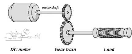
Fig. 1. Schematic of a simplified motion of attached load to DC motor

The transfer function of DC motor electric component relating input armature current, i a and voltage V in , can be derived by applying Kirchoff’s law around the electrical loop by summing voltages throughout the R-L circuit, this gives (1), taking Laplace transform and rearranging gives (2):

£ V = V _m — V r — V l — EMF = 0 (1)

Vin

= R * ia

+ ^La

di)     d9

- 1 + Kb dt)      dt

The electrical and mechanical components of PMDC motor are coupled to each other through an algebraic torque equation given by:

To derive the PMDC motor transfer function, we need to rearrange (2) describing electrical characteristics of PMDC, such that we have only I(s) on the right side, then substitute this value of I(s) in (6) describing PMDC mechanical characteristics, this all gives [4-6] :

( L a s + R a ) I ( s ) = V in ( s ) - K b S ^ ( s )

I . ( s ) =

(L.s + R.)

[ V an ^{( s} ) - ^Kb . ^{( s} ) ]

I - ( s )       ₌        1

[ V in ( s ) - K , . ( s ) ]    [ ( L . s + R a )

K t

Transfer function of PMDC motor mechanical

(L.s + R.)

[ V an ( s ) - K b . ( s ) ]

component relating output torque , T m and input rotor speed is derived by performing the energy balance; the sum of the torques must equal zero, we have (3) Substituting, and rearranging, we have (4):

£ t = J

*a = J *

Rearranging (8), we obtain the PMDC motor open loop transfer function without any load attached relating the input voltage, V_an(s), to the motor shaft output angle, 6(s) , given by:

T e — T , — T . — T EMF = 0

K t * a. = T a + T . + ( T oad + T f )

^G.ngle ^{( s} ) =

9 ( s )

V in ( s )

Where T f : The coulomb, can be found at steady state, where derivatives are zero, to be[5] :

K * ia - b * . = T

^Kt                            (9)

{ s [ ( L . s + R . )( J m s + b m ) + K t K ₅ ] }

K t

L . J m s ³ + ( R . J m + b m L . ) s ³ + ( R . b m + K_K b ) s

In the following calculation the disturbance torque, T, is all torques including coulomb friction, can be for simplicity assumed zero , and T is given by; T=T_load+T_f . Substituting in (4) each of (5) and the following values: T e = K^a . , T_a = J m *d²6/dt² , T „ = b m *d6/dt , and considering that in the open loop DC motor system without load attached, the change in T load is zero gives :

The PMDC motor open loop transfer function relating the input voltage, V in (s), to the angular velocity, ω(s), given by:

^Gspeed ^{( s} ) =

. ( s )

V in ( s )

Taking Laplace transform and rearranging gives:

K . I ( s ) - T oad - J m S 2 9 ( s ) - b m S 9 ( s ) = 0 ^Kt I ( s ) - T load = ( J m s ^{+ b}m ) s ⁹ ( s )

^Kt                          (10)

{[(L.s + R.)(Jms + bm) + KtKb ]}

K t

L . J m s ² + ( R . J m + b m L . ) s + ( R . b m + K , K b )

. ( s )

[ K_tI . ( s ) - T Load ( s ) ]

(Jms + bm )

In case of no load attached, T load =0, we have:

. ( s )

[ K t I . ( s ) ]

(Jms + bm )

Here note that the transfer function G angle (s) can be expressed as: Ga ( s ) =G_speed ( s ) *(1/s) . This can be obtained using MATLAB, using the following, code [1]:

>> G_angle = tf(1,[1,0] )* G_speed

Where: running tf(1,[1,0] ), will return 1/s

III. Controller Selection And Design

The modern advances in electric motors and controllers improve motors speed, acceleration, controllability, and reliability; also allow designers a wider choice of power

and torque. The term control system design refers to the process of selecting feedback gains that meet design specifications in a closed-loop control system. Most design methods are iterative, combining parameter selection with analysis, simulation, and insight into the dynamics of the plant [2]. There are many motor motion control strategies that may be more or less appropriate to a specific type of application each has its advantages and disadvantages. The designer must select the best one for specific application. 1n [2-3] most suitable control strategies for DC motor motion control, are suggested, were different control strategies were selected, designed, applied and their action were compared to select the most suitable control of a given DC motor in terms of output speed and angle, Most of these suggested control strategies will be applied in suggested system model, mainly PID, PI, PD as separate blocks to be applied with and without deadbeat response, also lead and lag compensators, the designer must select the best controller for specific application.

PID controller design: PID controllers are most used to regulate and direct many different types of dynamic plants the time-domain, The PID gains are to be designed and tuned to obtain the desired overall desired response. The PID controller transfer function is given by:

Rearranging, we have the following form:

G p _D ( s ) = - p + -_Ds = -_D ( s + I P )

- D ( s + Z pd ) ^ Z pd =

The PD-controller is equivalent to the addition of a simple zero at Z PD :

Lead compensator: Lead compensator is a soft approximation of PD-controller, The PD controller, given by G PD (s) = K P + K D s , is not physically implementable, since it is not proper, and it would differentiate high frequency noise, thereby producing large swings in output, to avoid this, PD-controller is approximated to lead controller of the following form[6,7,8]:

G pD ( s ) - G Lead ( s ) = - p + - D

Ps s + p

The larger the value of P , the better the lead controller approximates PD control, rearranging gives:

, .            _ Ps

G_Lead ( s ) = - p + -d—-

Gpid = Kp + -I- + Kd

K_Ds ² + K_Ps + -

-P (s + p) + -Dps

K D

² + K p

K D

K I

K D

(-p + -Dp) s + -pp s + p

Proportional -Integral (PI) - PI controller is widely used in variable speed applications and current regulation of electric motors, because of its simplicity and ease of design. PI controller transfer function is given by:

s += ( -p + -dp ) —

-p + -dp s + p

K, (-_Ps + - J

KPP

Now, let - = - + - p and Z = ----------- ,

C p D          (-p + -dp )

we obtain the following approximated controller transfer function of PD controller , and called lead compensator:

K P

-P (s + Zo)

G ( s ) = - C

s + Z s + p

s

Where, Zo: Zero of the PI-controller, K_P: The proportional gain, K_PI: The proportional coefficient; T_I: time constant. This transfer function, shows that, PI controller represents a pole located at the origin and a stable zero placed near the pole, at Z o =- K I / K P , resulting in drastically eliminating steady state error due to the fact that the feedback control system type is increased by one.

Proportional -Derivative , PD controller: The transfer function of PD-controller is given by :

^G pD ⁽ s ) = ^- P ^{+ -} D s

If Z < P this controller is called a lead controller (or lead compensator). If Z > P: this controller is called a lag controller (or lag compensator) .The transfer function of lead compensator is given by:

(s + Z )

G_M ( s ) = - c , Where : Z_o <  p_o   (14)

(s + p0 )

Lag compensator; The Lag compensator is a soft approximation of PI controller, it is used to improve the steady state response, particularly, to reduce steady state error of the system, the reduction in the steady state error accomplished by adding equal numbers of poles and zeroes to a systems [7].

G pi ( s ) - G ag ( s ) = K p + K = K P s + K ss

= K P

s

Since PI controller by it self is unstable, we approximate the PI controller by introducing value of P_o that is not zero but near zero; the smaller we make P o , the better this controller approximates the PI controller, and

(s + Z )

^G^g ⁽ s ) = ^Kc ⁽¹⁵⁾

Where: Z_o > P_o, and Z_o small numbers near zero and Z_o =K I /K P , the lag compensator zero. P o : small number ,The smaller we make P o , the better this controller approximates the PI controller.

• 3.1    Sensors modeling: speed and position Sensors

To close the control loop, the output of PMDC, needs to be measured and fedback to control system. The sensing device used to measure and feedback the output actual position of the motor shaft, is potentiometer. The potentiometer output is proportional to the motor shaft angle, θ, The output voltage of potentiometer, V pot is given by: V_pot = θ_a * K_pot . The potentiometer constant, K_pot equals the ratio of the voltage change to the corresponding angle change,

For robot arm, Potentiometer is used to measure the actual output arm position, θ L ,and convert it into corresponding volt, V p and then feeding back this value to controller, the Potentiometer output is proportional to the actual robot arm position, θ L . An applied voltage of 0 to 12 volts corresponds linearly to an output arm angle of 0 to 180, this gives the potentiometer constant, K_pot equals:

_ (Voltage change) _ ( 12 - 0 )

^pot (Degree change) ( 180 - 0 )      (16)

= 0.0667 V / degree

For mobile robot, Tachometer is used to measure the actual output angular speed, ω . . Dynamics of tachometer can be represented using (16), correspondingly, the transfer function of the tachometer is given by (17), We are to drive a given robotic platform system, using a given PMDC, with linear velocity of 0.5 m/s, the angular speed is obtained as: ω=V/r = 0.5/ 0.075 = 6.6667 Rad/s. Substituting values, we have Tachometer constant, given by (18):

d 9 (t)   „   .

V — Vout ⁽ s )

~^ K tach

to( s )

Kach = ^2— = 1-8- tach 6.6667

The following nominal values for the various parameters of a PMDC motor used : V_in=12 Volts; J m =0.02 kg·m²,; b m =0.03; K t =0.023 N-m/A ; K b =0.023 V-s/rad, R a =1 Ohm ; and L a =0.23 Henry; T L = no load attached , gear ratio, n=1:2, and design criteria : applied voltage of Vin = 0 to 12 volts corresponds linearly to an output arm angle θ =0 to 180, PO% < 5%, T s < less 2 second, gain margin, G m > 20 dB, phase margin, Φ m > 40 degrees, Ess =0. A negative feedback control system with forward controller shown in Figure 2(a)(b) is used

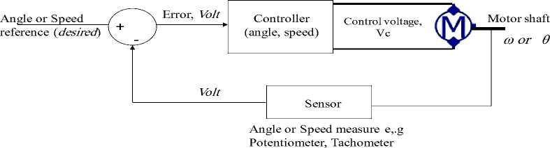
Fig.2(a) Block diagram representation of PMDC motor control

Controller to be         PMDC Motor selected and designed       Subsystem

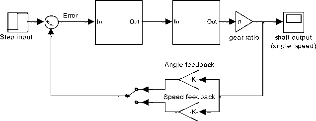
Fig. 2(b). Preliminary Simulink model for negative feedback with forward compensation

• 3.2    Simulink model and built-in function

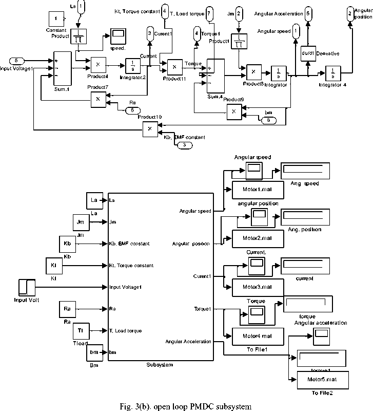
The derived transfer function can be used to built a Simulink model show in Figure 3(a), this model has, allmostly, the same functions as the designed and proposed built-in function, open loop models and subsystems of PMDC motor shown in Figure 3(b)(c) can also be used to replace dc motor in block given in Figure 3(a), using manual switch designer can select controller type and output controlled variable ( speed or angle) .

To simplify and accelerate the performance analysis of open loop motor system, as well as select and design a control system, a new MATLAB function is designed, named pmdc , this function is called by typing it in command window as any MATLAB built-in function, it has no input argument, when function is called, first designer is asked to define used PMDC motor parameters, time vector for output speed and angle response and finally desired output both maximum angle ( for position control application), and speed ( for speed control application), in result built-in function will return , potentiometer constant, tachometer constant, PMDC motor open loop transfer function in terms of input voltage and output angle, output speed, and corresponding step, ramp parabolic responses, second designer is asked to select control system (Pro,D,I, PI,PD, PID, lag, lead ,lead integral), and corresponding gains values in row vector form, in result MATLAB will return the step response of output speed and angle , and display in both tabular and curve forms the system performance specifications with selected controller applied, Finally to select more suitable control system and compare applying any controller the program once again, ask user to select another controller type, and return the same result but for the new controller selected.

The selected control system response can by verified and once again evaluated, by defining the selected gains and zeros and running Simulink model. To demonstrate how the proposed function works, the following nominal values of a given DC motor are to be used: Vin= 12; Jm=0.02; bm =0.03; Kt =0.023; Kb=0.023 ;Ra =1;La=0.23; TL = 0; maximum desired output angle=180 ( in positron control) ;max desired output speed=6.6667 ( motion control) ; potentiometer constant Kpot =0.0667 ; tachometer constant Ktach=1.8;

• IV.    Demonstrations, Testing And Results

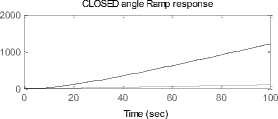
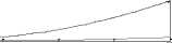
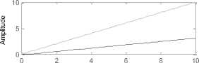
Running the proposed built in function for given motor parameters and choosing time vector for output angle and speed responses to be correspondingly: [0:0.1:10] and [0:0.1:100], then by defining nominal values of used PMDC parameters and finally running the model, the model will return shown in Figure 4(a) open loop and closed loop PMDC system transfer functions and response curves, by studying and analyzing these curves we can see that both closed loop transfer functions in terms of both output angle and speed is type zero, with finite E ss for step input, and infinity E ss for both ramp and parabolic.

Now, selecting, PD controller and defining PD gains, for simplicity to be Kp = [1 2 3], Kd= [1 2 3], will result in step responses in terms of output speed and angle shown in Figure 4(b) and table of performance specifications values in terms of both output speed and angle shown below: next below is shown what will be seen in MATLAB command window when running the program and applying PD controller:

• V.    Design Verification Using New Built-In Function And Simulink Model

A new MATLAB function is designed, named pmdc, this function is called within MATLAB by typing it in command window as any MATLAB built-in function, it has no input argument, when function is called, first designer is asked to define used PMDC motor parameters, time vector for output speed and angle response and finally desired output both maximum angle( for position control application), and speed( for speed control application),, in result built-in function will return, potentiometer constant, tachometer constant, PMDC motor open loop transfer function in terms of input voltage and output angle then output speed, and corresponding step, ramp parabolic response, second designer is asked to select control system (Pro,D,I, PI,PD, PID, lag, lead ,lead integral), and corresponding gains values in row vector form ,and in result MATLAB will return the step response of output speed and angle , and display in both tabular and curve forms the system performance specifications after selected controller is applied, Finally to select more suitable control system and compare applying any controller the program once again. Ask used to select another controller type, and return the same result but for the new controller selected.

The selected control system response can by verified and once again evaluated, by defining the selected gains and zeros and running Simulink model. To demonstrate how the proposed function works, the following nominal values of a given DC motor are to be used: Vin= 12; Jm=0.02; bm =0.03; Kt =0.023; Kb=0.023 ;Ra =1;La=0.23; TL = 0; maximum desired output angle=180 ( in positron control) ;max desired output speed=6.6667 ( motion control); potentiometer constant Kpot =0.0667 ; tachometer constant Ktach=1.8;

• VI.    Demonstrations, Testing And Results

Running the proposed built in function for given motor parameters and choosing time vector for output angle and speed responses to be correspondingly: [0:0.1:10] and [0:0.1:100], then by defining ( entering) nominal values of used PMDC parameters and clicking enter, open loop and closed loop PMDC system transfer functions shown below and responses, shown in Figure 4(a) will be displayed, by studying these curves we can see that both closed loop transfer functions in terms of both output angle and speed is type zero, with finite E ss for step input, and infinity E ss for both ramp and parabolic.

Now, selecting, PD controller and defining PD gains, for simplicity to be Kp = [1 2 3], Kd= [1 2 3], will result in step responses in terms of output speed and angle shown in Figure 4(b) and table of performance specifications values in terms of both output speed and angle shown below: next below is shown what will be seen in MATLAB command window when running the program and applying PD controller:

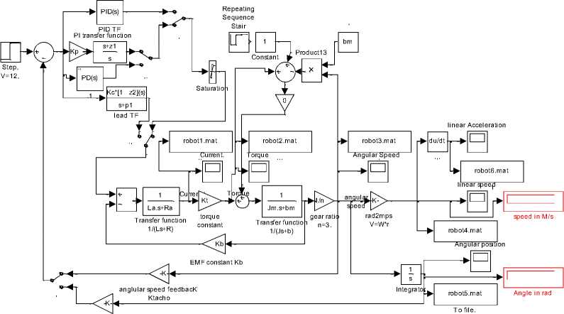
angle feedbacK Kpot

Fig. 3(a). Simulink model

Analysis and controller selection and evaluation of a given PMDC motor output Angle OR Speed :-Program

T(s) = 'Omega'(s)/Vin(s)=

0.023

0.0046 s^2 + 0.0269 s + 0.07193

Jm bm Kt Ra La Desired output Desired output Kpot Ktach angle       speed

0.02 0.03 0.023  1  0.23     180       6.6667

0.0666667  1.79999

Choose controller TYPE : Pro,D,I, PI,PD, PID, lag, lead ,lead integral :PD

Enter Proportional gain values in row vector form Kp = [1 2 3]

Enter Derivative gain values in row vector form Kd = [1 2 3]

Enter time vector for output speed response: [0:0.1:10]

Enter time vector for angle output response: [0:0.1:10]

For chosen Kp,Kd the following ANGLE RESPONSE SPEC. results are obtained:

G(s) = 'Theta'(s)/Vin(s)=

0.023

0.0046 s^3 + 0.0269 s^2 + 0.03053 s

Transfer function:

0.023

Gain	Gain	Error (Mp)  max Output	Final
Kp	Kd	(Ess)       Peak value	output
1.0000	1.0000	0.0900 -34.5487 145.4513	=17=9=.9=1=00= =
2.0000	2.0000	0.0900 -0.3713 179.6287	179.9100
3.0000	3.0000	0.0900 -0.0900 179.9100	179.9100

For chosen Kp,Kd the following ANGLE RESPONSE SPEC. results are obtained:

Gain Gain Error (Mp1) max value Final

Kp Kd (Ess1) (Mu1) (Peak) output

0.0046 s^3 + 0.0269 s^2 + 0.03053 s + 0.001534

G(s) = 'Omega'(s)/Vin(s)=

0.023

1.0000  1.0000  4.5913 -2.8035  3.8632  2.0754

2.0000  2.0000  2.3741 -1.6189  5.0478  4.2926

3.0000  3.0000  1.3154 -1.0650  5.6017  5.3513

Choose controller TYPE : Pro,D,I, PI,PD, PID, lag, lead ,lead integral:

0.0046 s^2 + 0.0269 s + 0.03053

Open loop PMDC motor system ,step ANGLE response

0        20       40       60       80       100

Time (sec)

CLOSED speed Step response 0.4

Time (sec)

_{x 10} ⁵ CLOSED angle Parabolic response 2

0       20

Time

CLOSED speed Ramp response

Time (sec)

Fig. 4(a). analyzing open and closed loop system response, closed loops system's responses to step ramp and parabolic inputs

40       60       80      100

Time

CLOSED speed Parabolic response

Time

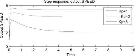
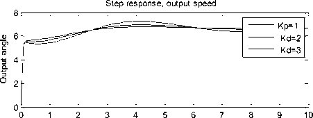
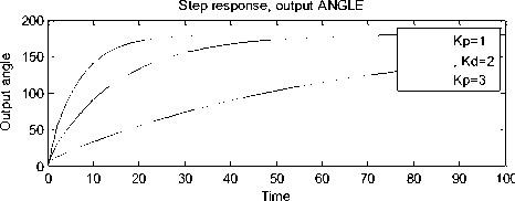
Fig. 4(b). closed loop system response, in terms of output speed and angle when PD controller is selected for Kp=Kd=[1 2 3]

Time

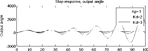
Fig. 6. response of PMDC motor when PID Controller is applied with K P =[ 1 2 3], K I =[ 1 2 3], K D =[ 1 2 3],

Running the proposed built-in function for given motor parameters and choosing Lead compensator with gains , for simplicity, Kc = [1 2 3], Z = [1 2 3] and P = [1 2 3], will return the up mentioned information, mainly compensator closed transfer function for each time each value of three vectors is substituted, as well as the response plots shown in Figure 5.

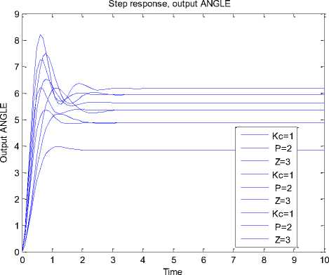
Fig. 5. response of PMDC motor when lead compensator is applied with the following different gains, poles and zeros : Kc = [1 2 3], Z = [1 2 3] and P = [1 2 3],

Running the proposed built-in function for given motor parameters and choosing PID controller with gains K P =[ 1 2 3], K I =[ 1 2 3], K D =[ 1 2 3], will return PID, and closed transfer function for each time each value of three vectors is substituted, will return the mentioned results and plots shown in Figure 6.

To verify design, calculations and built in function results, the proposed Simulink for given motor parameters and choosing PID controller with gains e.g. K P =[1], K I =[1], K D =[1], is used.

• VII.    The Set Of MATLAB New Proposed Built-In Function Instructions

function pmdc

% PMDC Used for a given PMDC Analysis and controller selection and evaluation of

%     a given PMDC motor desired output Angle OR Speed

%      There is no input argument, the function is called by by typing its name

%        Then select controller for performance analysis and design

%     Author : Dr Farhan Atallah Salem AbuMahfouz

%     Dtate : 10/02/2000

% clear all ;close all; clc disp(' ')

fprintf(' ---------------------------------------------------------\n')

fprintf('                 Analysis and controller selection and evaluation of \n')

fprintf('         a given PMDC motor output Angle OR Speed

:-Program \n')

fprintf(' --------------------------------------------------------\n')

fprintf('

=====================\n')

% Vin= 12;Jm=0.02;bm =0.03;Kt =0.023; Kb=0.023 ;Ra =1;La=0.23; TL = 0;max_angle=180;max_speed=6.6667 ;Kpot =0.0667 ;Ktach=1.8;

Jm = input(' Enter moment of inertia of the rotor, (Jm) =');

bm = input(' Enter damping constant of the mechanical system ,(bm)=');

Kt = input(' Enter torque constant, Kt=');

Kb = input(' Enter electromotive force constant, Kb=');

Ra = input('Enter electric resistance of the motor armature (ohms), Ra =');

La =input(' Enter electric inductance of the motor armature (Henry), La=');

Vin = input(' Enter Max. applied input voltage, Vin = '); max_angle=input(Enter Max. required output angle = ') ; max_speed=input(Enter Max. required output speed = ') linear_speed=input(' Enter desired robot linear speed ');

Kpot=Vin/max_angle;

Ktach= Vin/max_speed;

num1 = [1];den1= [La ,Ra];num2 = [1];den2= [Jm ,bm];

A = conv( [La ,Ra], [Jm ,bm]); TF1 =tf(Kt, A);

G_speed= feedback(TF1,Kb),G_angle=tf(1,[1,0] )*G_speed, fprintf('

==============\n')

fprintf(' PMDC Motor parameters: Jm= %g, bm=%g, Kt=%g,Ra=%g,La=%g,Desired angle=%g,Desired speed=%g : \n', Jm,bm,Kt,Ra,La,max_angle,max_speed) home fprintf(' -------------------------------------------------------- \n')

disp( ' Jm bm Kt Ra La Desired output Desired output Kpot Ktach ')

disp( '                    angle        speed ')

fprintf(' %g %g %g %g %g %g %g %g %g \n ',

Jm,bm,Kt,Ra,La,max_angle,max_speed,Kpot,Ktach)

disp(' -------------------------------------------------------------')

disp(' --------------------------------------------------------------')

G_open_motor_num=[Kt];

G_open_motor_speed_den= [La*Jm,    (Ra*Jm+bm*La),

(Ra*bm+Kt*Kb)];

G_open_motor_angle_den=[La*Jm,        (Ra*Jm+bm*La),

(Ra*bm+Kt*Kb), 0];

t1=input('Enter  time  vector  for  output speed  response

:');%t1=0:0.001:6;

t2=input('Enter  time  vector  for  angle  output  response

:');%0:0.001:150;

fprintf('

==================\n')

disp(' ')

fprintf(' G(s) = ''Theta''(s)/Vin(s)=\n ')

G_open_motor_angle=tf(Kt,[La*Jm,        (Ra*Jm+bm*La),

(Ra*bm+Kt*Kb), 0])

T_close_motor_angle=feedback(G_open_motor_angle,Kpot)

fprintf('

=================\n') fprintf('

==================\n')

disp(' ')

fprintf(' G(s) = ''Omega''(s)/Vin(s)=\n ')

disp(' ')

fprintf(' T(s) = ''Omega''(s)/Vin(s)=\n ')

T_closed_motor_speed=feedback(G_open_motor_speed,

Ktach)

fprintf('

=====================\n')

fprintf(' -------------------------------------------------------------\n')

subplot(4,3,2) ,step(Vin*G_open_motor_angle,t2), title(' Open loop PMDC motor system ,step ANGLE response '), ylabel('Output Angle '), xlabel('Time')

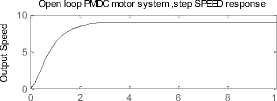
subplot(4,3,5) ,step(Vin*G_open_motor_speed,t1), title(' Open loop PMDC motor system ,step SPEED response '), ylabel('Output Speed'), xlabel('Time')

% output CLOSED loop angle response u = t2; u1 = t2 ;u2 = t2.*t2;

[y,x] = step(T_close_motor_angle,t2);

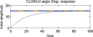
subplot(4,3,7) ,plot(t2,y,t2,15 ), xlabel('Time'), ylabel('Error amplitude') title(' CLOSED angle Step response') % [yy,xx] = lsim(T_close_motor_angle,u1,t2);

% subplot(4,3,8) ,plot(t2,yy,t2,u1)

subplot(4,3,8), lsim(T_close_motor_angle,u1,t2);

xlabel('Time'), ylabel(' ') %ylabel('Error amplitude') title(' CLOSED angle Ramp response')

[yyy,xxx] = lsim(T_close_motor_angle,u2,t2);

subplot(4,3,9) ,plot(t2,yyy,t2,u2)

xlabel('Time'), %ylabel('Error amplitude') title(' CLOSED angle Parabolic response')

% output CLOSED loop speed response uu = t1; uu1 = t1 ;uu2 = t1.*t1;

[N,M] = step(T_closed_motor_speed,t1);

subplot(4,3,10) ,plot(t1,N,t1,0.32 ), xlabel('Time'), ylabel('Error amplitude') title(' CLOSED speed Step response')

% [NN,MM] = lsim(T_closed_motor_speed,uu1,t1);

% subplot(4,3,11) ,plot(t1,NN,t1,uu1)

subplot(4,3,11), lsim(T_closed_motor_speed,uu1,t1);

xlabel('Time'), %ylabel('Error amplitude') title('CLOSED speed Ramp response')

[NNN,MMM] = lsim(T_closed_motor_speed,uu2,t1);

subplot(4,3,12) ,plot(t1,NNN,t1,uu2)

xlabel('Time'), %ylabel('Error amplitude') title('CLOSED speed Parabolic response') quit=1;

while quit~=0

disp(' ')

fprintf('================================= =====================\n');

controller=input('Choose controller TYPE : Pro,D,I, PI,PD, PID, lag, lead ,lead integral :', 's');

fprintf(' ------------------------------------------------------\n')

home disp(' '),disp(' ')

G_open_motor_speed=tf(Kt,[La*Jm,

(Ra*bm+Kt*Kb)])

(Ra*Jm+bm*La),

zz=lower (controller); switch (zz)

case 'pro'

Kp=input(' Enter proportional gain values in row vector form, Kp = ');% Kp =[ 1 5 8 ];

Ess_step=zeros(1,length(Kp));

angle_max=zeros(1,length(Kp));

angle_end=zeros(1,length(Kp));

for i=1:length(Kp)

Q=1:length(Kp);

G_close_P_speed= feedback(Kp(i)*G_open_motor_speed,Ktach);

G_close_P_angle                             = feedback(Kp(i)*G_open_motor_angle,Kpot);

y1(:,i)=step(Vin*G_close_P_speed,t1);

y2(:,i)=step(Vin*G_close_P_angle,t2);

%pause(1)

yA(:,i)=step(Vin*G_close_P_angle,t2.*1000);

angle_endA(Q(i))= yA(end);

angle_max(Q(i))= max(y2(:,i));

Ess_step(Q(i))=                              1/(1+ dcgain(Kp(i).*G_open_motor_angle));

Ess(i) = max_angle - angle_end(Q(i));

Mp(i)= angle_max(Q(i))- max_angle;

yB(:,i)=step(Vin*G_close_P_speed,t1.*1000);

speed_endA(Q(i))= yB(end);

speed_max(Q(i))= max(y1(:,i));

Ess1_step(Q(i))=                             1/(1+ dcgain(Kp(i).*G_open_motor_speed));

Ess1(i) = max_speed - speed_endA(Q(i));

Mp1(i)= speed_max(Q(i))- max_speed;

end figure, subplot(2,1,1),plot(t1,y1(:,1:length(Q)));

title('Closed loop Step response, output SPEED   '),ylabel('

Output SPEED'),xlabel('Time')

C = regexp(sprintf('Kp=%d#', Kp), '#', 'split'); C(end) = []; legend( C ), ylabel(' Output speed'), subplot(2,1,2),plot(t2,y2(:,1:length(Q))), legend(C ) title('Closed loop Step response, output ANGLE

'),ylabel(' Output angle'),xlabel('Time')

%figure, sisotool(Kp(i)*G_close_P_speed) fprintf('   \n');

fprintf('================================= ====================\n');

fprintf('For chosen Kp, the following ANGLE RESPONSE SPEC. results are obtained: \n');

fprintf('================================= ========================\n');

fprintf(' Gain Error (Mp) max value Final \n');

fprintf(' Kp (Ess) (Mu) (Peak) output \n');

fprintf(' ---------------------------------------------------------\n')

answers= [Kp' Ess' Mp' angle_max' angle_endA' ];

disp(answers )

fprintf('================================= =======================\n');

fprintf('=================================

=========================\n');

fprintf('For chosen Kp, the following SPEED RESPONSE SPEC. results are obtained: \n');

fprintf('================================= ========================\n');

fprintf(' Gain Error (Mp1) max value Final \n');

fprintf(' Kp (Ess1) (Mu1) (Peak) output \n');

fprintf('================================= ========================\n');

answers= [Kp' Ess1' Mp1' speed_max' speed_endA' ];

disp(answers )

fprintf('================================= =========================\n');

case 'd'

Kd =input(' Enter Derivative gain values in row vector form Kd = ');%[700 750 800];

Ess_step=zeros(1,length(Kd));

angle_max=zeros(1,length(Kd));

angle_end=zeros(1,length(Kd));

for i=1:length(Kd)

Q=1:length(Kd);

G_d=[Kd(i) 0];

numa=G_d*Kt;

G_open_D_speed=tf(numa,G_open_motor_speed_den );

G_open_D_angle=tf(numa,G_open_motor_angle_den );

G_close_D_speed=feedback(G_open_D_speed,Ktach);

G_close_D_angle=feedback(G_open_D_angle,Kpot) y1(:,i)=step(Vin*G_close_D_speed,t1);

y2(:,i)=step(Vin*G_close_D_angle,t2);

% calculating output Angle response specification yA(:,i)=step(Vin*G_close_D_angle,t2.*100); angle_end(Q(i))= y2(end);

angle_endA(Q(i))= yA(end);

angle max(Q(i))=max(y2(:,i));

Ess_step(Q(i))=                              1/(1+ dcgain(Kd(i).*G_open_D_angle));

Ess(i) =max_angle - angle_endA(Q(i)) ;

Mp(i)= angle_max(Q(i))- max_angle;

% calculating output Speed response specification yB(:,i)=step(Vin*G_close_D_speed,t1.*1000);

speed_endA(Q(i))= yB(end);

speed_max(Q(i))= max(y1(:,i));

Ess1_step(Q(i))=                             1/(1+ dcgain(Kd(i).*G_open_motor_speed));

Ess1(i) = max_speed - speed_endA(Q(i));

Mp1(i)= speed_max(Q(i))- max_speed;

end subplot(2,1,1),plot(t1,y1(:,1:length(Q)));title('Step response, output SPEED '),ylabel(' Output SPEED'),xlabel('Time')

C = regexp(sprintf('Kd=%d#', Kd), '#', 'split'); C(end)=[]; legend( C ), subplot(2,1,2),plot(t2,y2(:,1:length(Q))), legend(C ), title('Step response,    output ANGLE         '),ylabel('    Output angle'),xlabel('Time')

fprintf('   \n');

fprintf('================================= =========================\n');

fprintf('For chosen Kd, the following ANGLE RESPONSE SPEC. results are obtained: \n');

fprintf('================================= ========================\n');

fprintf(' Gain Error (Mp) max Ouput Final \n');

fprintf(' Kd (Ess)       Peak value output \n');

fprintf('================================= ==========================\n');

answers= [Kd' Ess' Mp' angle_max' angle_endA' ];

disp(answers )

fprintf('================================= ==========================\n');

fprintf('================================= =========================\n');

fprintf('For chosen Kp, the following SPEED RESPONSE SPEC. results are obtained: \n');

fprintf('================================= ==========================\n');

fprintf(' Gain Error (Mp1) max value Final \n');

fprintf(' Kp (Ess1) (Mu1) (Peak) output \n');

fprintf('================================= ========================\n');

answers= [Kd'     Ess1'    Mp1'     speed_max'

speed_endA' ];

disp(answers )

fprintf('================================= =======================\n');

case 'i'

Ki =input(' Enter Derivative gain values in row vector form Ki = '),%[0.009 1  3];

Ess_step=zeros(1,length(Ki));

angle_max=zeros(1,length(Ki));

angle_end=zeros(1,length(Ki));

for i=1:length(Ki)

Q=1:length(Ki);

num_G_I=[Ki(i)];

den_G_I=[1 0];

G_I=tf(num_G_I,den_G_I);

G_open_I_speed_num=conv(num_G_I,G_open_motor_num);

G_open_I_speed_den=conv(den_G_I,G_open_motor_speed_de n);

G_open_I_speed

=tf(G_open_I_speed_num,G_open_I_speed_den );

G_open_I_angle_num=conv(num_G_I,G_open_motor_num);

G_open_I_angle_den=conv(den_G_I,G_open_motor_angle_de n);

G_open_I_angle

=tf(G_open_I_angle_num,G_open_I_angle_den );

G_close_I_speed=feedback(G_open_I_speed,Ktach); G_close_I_angle=feedback(G_open_I_angle,Kpot);

% calculating output Angle response specification y1(:,i)=step(Vin*G_close_I_speed,t1);

y2(:,i)=step(Vin*G_close_I_angle,t2);

%pause(1)

yA(:,i)=step(Vin*G_close_I_angle,t2.*100);

angle_end(Q(i))= y2(end);

angle_endA(Q(i))= yA(end);

angle max(Q(i))=max(y2(:,i));

Ess_step(Q(i))=                              1/(1+ dcgain(Ki(i).*G_open_I_angle));

Ess(i) =max_angle - angle_endA(Q(i)) ;

Mp(i)= angle_max(Q(i))- max_angle;

% calculating output speed response specification yB(:,i)=step(Vin*G_close_I_speed,t1.*1000); speed_endA(Q(i))= yB(end);

speed_max(Q(i))= max(y1(:,i));

Ess1_step(Q(i))=                             1/(1+ dcgain(Ki(i).*G_open_I_speed));

Ess1(i) = max_speed - speed_endA(Q(i));

Mp1(i)= speed_max(Q(i))- max_speed;

end subplot(2,1,1),plot(t1,y1(:,1:length(Q)));

title('Step response, output SPEED '),ylabel(' Output

SPEED'),xlabel('Time')

C=regexp(sprintf('Kd=%d#',       Ki),        '#',        'split');

C(end)=[];legend(C ),subplot(2,1,2),plot(t2,y2(:,1:length(Q))), legend(C ), title('Step response, output ANGLE '),ylabel(' Output angle'),xlabel('Time'), format short, fprintf(' \n');

fprintf('================================= ========================\n');

fprintf('For chosen Ki, the following ANGLE response spec. results are obtained: \n');

fprintf('================================= =========================\n');

fprintf(' Gain Error (Mp) max output Final \n');

fprintf(' Ki (Ess)      Peak value output \n');

fprintf('================================= =========================\n');

answers= [Ki' Ess_step' Mp' angle_max' angle_endA' ];

disp(answers )

fprintf('================================= ========================\n');

fprintf('================================= ========================\n');

fprintf('For chosen Kp, the following SPEED response spec. results are obtained: \n');

fprintf('================================ =========================\n');

fprintf(' Gain Error (Mp1) max value Final \n');

fprintf(' Kp (Ess1) (Mu1) (Peak) output \n');

fprintf('================================ =========================\n');

answers= [Ki' Ess1' Mp1' speed_max' speed_endA' ];

disp(answers )

fprintf('================================= =========================\n');

fprintf(' The I-controller has the unique ability to return \n')

fprintf(' the process back to the exact setpoint that is eliminating \n')

fprintf(' the error, but it has a disadvantage based on fact that integration \n')

fprintf(' is a continual summing. Integration of error over time means summing \n')

fprintf(' up the complete controller error history up to the present time, this means\n')

fprintf(' I-controller can initially allow a large deviation at the instant the error is \n')

fprintf(' produced. This can lead to system instability and cyclic operation \n')

case 'pd'

Kp =input('Enter Proprtinal gain values in row vector form Kp = ');%[1, 1.5 , 1.8703 ];

Kd=input('Enter Derivative gain values in row vector form Kd = ');%[ 1,2,3.336 ]

Ess_step=zeros(1,length(Kd));

angle_max=zeros(1,length(Kd));

angle_end=zeros(1,length(Kd));

for i=1:length(Kp)

Q=1:length(Kp);
for ii=1:length(Kd) G_PD=Kd(i)*[1 ,Kp(i)/Kd(ii)]; num=conv(G_PD ,Kt ); G_open_PD_speed=tf    (num,[La*Jm,	(Ra*Jm+bm*La),
(Ra*bm+Kt*Kb)]); G_open_PD_angle=tf    (num,[La*Jm,	(Ra*Jm+bm*La),
(Ra*bm+Kt*Kb), 0]);

G_close_PD_speed=feedback(G_open_PD_speed,Ktach);

G_close_PD_angle=feedback(G_open_PD_angle,Kpot);

y1(:,i)=step(Vin*G_close_PD_speed,t1);

y2(:,i)=step(Vin* G_close_PD_angle,t2); %pause(1)

yA(:,i)=step(Vin.*G_close_PD_angle,t2.*1000);

angle_end(Q(i))= y2(end);

angle_endA(Q(i))= yA(end);

angle_max(Q(i))=max(y2(:,i));

Ess_step(Q(i))=

1/(1+dcgain(Kd(i).*G_open_PD_angle));

Ess(i) =max_angle - angle_endA(Q(i)) ;

Mp(i)= angle_max(Q(i))- max_angle;

% calculating output speed response specification yA1(:,i)=step(Vin.*G_close_PD_speed,t1.*1000);

speed_end(Q(i))= y1(end);

speed_max(Q(i))=max(y1(:,i));

speed_endA(Q(i))= yA1(end);

Ess_step(Q(i))=

1/(1+dcgain(Kd(i).*G_open_PD_speed));

Ess1(i) =max_speed - speed_endA(Q(i)) ;

Mp1(i)= speed_max(Q(i))- max_speed; end end subplot(2,1,1),plot(t1,y1(:,1:length(Q)));title('Step response, output SPEED '),ylabel(' Output SPEED'),xlabel('Time'), C=regexp(sprintf('Kp=%g#,  Kd=%g#', Kp,Kd), '#', 'split');

C(end)=[];legend(C), subplot(2,1,2),plot(t2,y2(:,1:length(Q))), legend(C ),title('Step response,    output ANGLE         '),ylabel(' Output angle'),xlabel('Time')

fprintf('  \n');

fprintf('================================= =======================\n');

fprintf('For chosen Kp,Kd the following ANGLE RESPONSE SPEC. results are obtained: \n');

fprintf('================================= ======================\n');

fprintf(' Gain     Gain     Error (Mp)    max Output

Final \n');

fprintf(' Kp     Kd (Ess)        Peak value     output

\n');

fprintf('================================= =========================\n');

answers= [Kp'    Kd'     Ess'      Mp'     angle_max'

angle_endA' ];

fprintf('For chosen Kp,Kd the following ANGLE RESPONSE SPEC. results are obtained: \n');

fprintf('================================= ==========================\n');

fprintf(' Gain Gain Error (Mp1) max value Final \n');

fprintf(' Kp Kd (Ess1) (Mu1) (Peak) output \n');

fprintf('================================= ====================\n');

aanswers= [ Kp' Kd' Ess1'    Mp1' speed_max'

speed_endA' ];

disp(aanswers )

fprintf('================================= ======================\n');

case 'lead'

Kc =input('Enter Lead gain values in row vector form Kc = ');%[34,300,450 ];

Z=input('Enter Lead zero value , Z = ');%[ 1.5410];

P=input('Enter Lead Pole value , P = '); %[15.410]

Ess_step=zeros(1,length(Kc));

angle_max=zeros(1,length(Kc));

angle_end=zeros(1,length(Kc));

figure for i=1:length(Kc)

for ii=1:length(Z)

for iii=1:length(P)

Q=1:length(Kc);

num_lead= Kc(i).*[ 1 Z(ii)];

den_lead= [ 1 P(iii)];

disp(' Lead Transfer function : ') G_lead=tf(num_lead,den_lead) G_open_lead_speed=series                (G_lead

,G_open_motor_speed);

G_open_lead_angle=series                (G_lead

,G_open_motor_angle);

disp(' Closed loop Transfer function, SPEED/Vin= : ')

G_close_lead_speed=feedback(G_open_lead_speed,Ktach) disp(' Closed loop Transfer function, ABLE/Vin= : ')

G_close_lead_angle=feedback(G_open_lead_angle,Kpot) y1(:,iii)=step(Vin*G_close_lead_speed,t1);

y2(:,iii)=step(Vin*G_close_lead_angle,t2);

% pause(1)

yA(:,iii)=step(Vin*G_close_lead_angle,t2.*1000);

plot(t1,y1(:,1:length(Kp))) hold on title('Step response, output ANGLE     '),ylabel(' Output

ANGLE'),xlabel('Time'),C=regexp(sprintf('Kc=%d# P=%d# Z=%d#', Kc,P,Z), '#', 'split'); C(end)=[];legend(C ), angle_end(iii)= y2(end);

angle_endA(iii)= yA(end); angle_max(iii)=max(y2(:,iii));

Ess_step(iii)=                                  1/(1+ dcgain(Kc(i).*G_close_lead_angle));

Ess(iii) =angle_max(iii) - angle_endA(iii) ;

Mp(iii)= angle_max(iii)- max_angle; end end end case 'lead integral'

Kc =input('Enter Lead-Integral gain values in row vector form Kc = ');%[4 7 30 ];

Z=input('Enter Lead-Integral zero , Z =  ');%[

0.15410];

P=input('Enter Lead-Integral Pole , P = '); %[1.5410];

Ess_step=zeros(1,length(Kc));

angle_max=zeros(1,length(Kc));

angle_end=zeros(1,length(Kc));

for i=1:length(Kc)

Q=1:length(Kc);

num_lead= Kc(i)*[ 1 Z];

den_lead_integral= conv([1 0],[ 1 P]);

G_lead_integral=tf(num_lead,den_lead_integral);

G_open_controller_speed=series   (G_lead_integral

,G_open_motor_speed)

G_open_controller_angle=series   (G_lead_integral

,G_open_motor_angle)

G_close_controller_speed=feedback(G_open_controller_speed, Ktach);

G_close_controller_angle=feedback(G_open_controller_angle, Kpot)

y1(:,i)=step(Vin*G_close_controller_speed,t1); y2(:,i)=step(Vin*G_close_controller_angle,t2); %pause(1)

yA(:,i)=step(Vin*G_close_controller_angle,t2.*1000);

angle_end(Q(i))= y2(end);

angle_endA(Q(i))= round(yA(end));

angle max(Q(i))=max(y2(:,i));

Ess_step(Q(i))=                              1/(1+ dcgain(Kc(i).*G_open_controller_angle));

Ess(i) =max_angle - angle_endA(Q(i)) ;

Mp(i)= angle_max(Q(i))- max_angle;

end subplot(2,1,1),plot(t1,y1(:,1:length(Q)));

title('Step response, output SPEED '),ylabel(' Output SPEED'),xlabel('Time')

C = regexp(sprintf('Kd=%d#', Kc), '#', 'split'); C(end) = []; legend( C ), subplot(2,1,2),plot(t2,y2(:,1:length(Q))), legend(C ) title('Step response, output ANGLE '),ylabel(' Output angle'),xlabel('Time')

fprintf('   \n');

fprintf('================================\n' );

fprintf('For chosen Kc the following ANGLE RESPONSE SPEC. results are obtained: \n');

fprintf('=================================\ n');

fprintf(' Gain Error (Mp) max Output Final \n');

fprintf(' Kc (Ess)        Peak value output \n');

fprintf('=================================\ n');

answers= [Kc'       Ess'      Mp'     angle_max'

angle_endA' ];

disp(answers )

fprintf('=================================\ n');

case 'PI'

Ki=input('Enter Integral gain Ki = ');%[ 0.01];

Kp=input('Enter Proprtional gain Kp = ');% [9];

Z =[Ki/Kp];

num_PI=Kp*[1 Z];

den_PI=[ 1 0];

G_PI =tf(num_PI,den_PI)

G_open_PI_speed_num=conv(num_PI,Kt)

G_open_PI_speed=series(G_PI,G_open_motor_speed) G_open_PI_angle=series(G_PI,G_open_motor_angle) G_close_speed=feedback(G_open_PI_speed,1);

G_close_angle=feedback(G_open_PI_angle,Kpot) subplot(2,1,1),step(Vin*G_close_speed);

title('Step response, output speed '), [a,b]=step(Vin*G_close_angle,t1);

subplot(2,1,2), plot(t2,a), title('Step response, output angle ')

[yA,b]=step(Vin*G_close_angle,t2.*100);

angle_end= yA(end);

angle_endA = round(yA(end)) ;

angle_max = max(yA);

Ess =max_angle - angle_endA ;

Mp = angle_max - max_angle;

fprintf('   \n');

fprintf('=================================\ n');

fprintf('For chosen Kp,Ki, the following ANGLE RESPONSE SPEC. results are obtained: \n');

fprintf('=================================\ n');

fprintf(' Gain Gain Error (Mp) max output Final \n');

fprintf(' Kp    Ki (Ess)      Peak value output \n');

fprintf('=================================\ n');

answers= [Kp' Ki' Ess' Mp' angle_max' angle_endA' ]; disp(answers )

fprintf('=================================\ n');     case 'lag'

Kc =input('Enter lag compensator gain values in row vector form Kc = ');%[4 7 30 ];

Z=input('Enter lag zero , Z = ');%[ 0.13410];

P=input('Enter lag Pole , P = '); %[0.013410]

for i=1:length(Kc)

Q=1:length(Kc);

num_lag= Kc(i)*[ 1 Z];

den_lag= [ 1 P];

G_lag=tf(num_lag,den_lag);

G_open_lag_speed=series                  (G_lag

,G_open_motor_speed)

G_open_lag_angle=series                  (G_lag

,G_open_motor_angle)

G_close_lag_speed=feedback(G_open_lag_speed,Ktach);

G_close_lag_angle=feedback(G_open_lag_angle,Kpot) y1(:,i)=step(Vin*G_close_lag_speed,t1);

y2(:,i)=step(Vin*G_close_lag_angle,t2);

%pause(1)

yA(:,i)=step(Vin*G_close_lag_angle,t2.*100);

angle_end(Q(i))= y2(end);

angle_endA(Q(i))= round(yA(end));

angle max(Q(i))=max(y2(:,i));

Ess_step(Q(i))=                              1/(1+ dcgain(Kc(i).*G_open_lag_angle));

Ess(i) =max_angle - angle_endA(Q(i)) ;

Mp(i)= angle_max(Q(i))- max_angle;

end subplot(2,1,1),plot(t1,y1(:,1:length(Q)));

title('Step response, output speed '),

C = regexp(sprintf('Kc=%d#', Kc), '#', 'split'); C(end) = []; legend( C ), ylabel(' Output angle')

subplot(2,1,1),plot(t2,y2(:,1:length(Q))); title('Step response, output angle ')

legend( C ) ,ylabel(' Output angle'),xlabel('Time') fprintf('   \n');

fprintf('=================================\ n');

fprintf('For chosen Kc, the following ANGLE RESPONSE SPEC. results are obtained: \n');

fprintf('=================================\ n');

fprintf(' Gain Error (Mp) max output     Final \n');

fprintf(' Kc (Ess)       Peak value output \n');

fprintf('=================================\ n');

answers= [Kc',Ess', Mp' angle_max',angle_endA' ]; disp(answers )

fprintf('=================================\ n');

case 'pid'

Kp=input('Enter PID Proportional gain Kp =');%150 ;

Ki=input('Enter PID Integral gain Ki =');%11

Kd =input('Enter PID Derivative gain values in row vector form Kd = ');%[50 75 140];

% Z1=[ 4.3069]; Z2= [0.15410];

for i=1:length(Kp)

for ii=1:length(Ki)

for iii=1:length(Kd)

Q=1:length(Kd);

num_PID= Kd(iii)*[1 Kp(i)/Kd(iii) Ki(ii)/Kd(iii)]

den_PID= [ 1 0];

G_PID=tf(num_PID,den_PID);

G_open_PID_speed=series               (G_PID

,G_open_motor_speed);

G_open_PID_angle=series               (G_PID

,G_open_motor_angle);

G_close_PID_speed=feedback(G_open_PID_speed,Ktach);

G_close_PID_angle=feedback(G_open_PID_angle,Kpot) y1(:,i)=step(Vin*G_close_PID_speed,t1);

y2(:,i)=step(Vin*G_close_PID_angle,t2); pause(1)

angle_end(Q(i))= y2(end); angle_max(Q(i))=max(y2(:,i));

Ess_step(Q(i))= 1/(1+ dcgain( G_open_PID_angle)); yA(:,i)=step(Vin*G_close_PID_angle,t2.*100);

angle_end(Q(i))= y2(end);

angle_endA(Q(i))= round(yA(end));

angle max(Q(i))=max(y2(:,i));

Ess_step(Q(i))=                              1/(1+ dcgain(Kd(i).*G_open_PID_angle));

Ess(i) =max_angle - angle_endA(Q(i)) ;

Mp(i)= angle_max(Q(i))- max_angle; end end end plot(t1,y1(:,1:length(1)))

hold on, title('Step response, output ANGLE '),ylabel(' Output ANGLE'),xlabel('Time')

C=regexp(sprintf('Kp=%d# Ki=%d# Kd=%d#', Kp,Ki,Kd), '#', 'split');                                     C(end)=[];legend(C

),subplot(2,1,1),plot(t1,y1(:,1:length(Q)));

title('Step response, output speed '),

C = regexp(sprintf('Kp=%d# Kd=%i# Kd=%d#', Kd,Ki,Kp), '#', 'split'); C(end) = []; legend( C ),ylabel(' Output angle'), subplot(2,1,2),plot(t2,y2(:,1:length(Q)));title('Step response, output angle     '),   legend( C     ) ,ylabel(' Output angle'),xlabel('Time ') fprintf('   \n');

fprintf('=================================\ n');

fprintf('For chosen Kp=%d Ki=%d and Kd=%d, the following ANGLE RESPONSE SPEC. results are obtained: \n', Kp ,Ki, Kd);

fprintf('=================================\ n');

fprintf(' Gain Error (Mp) max output Final \n');

fprintf(' Kd (Ess)      Peak Value output \n');

fprintf('=================================\ n');

answers= [Kd',Ess', Mp' ,angle_max',angle_endA' ];

disp(answers                                                 ), fprintf('=================================\ n');

otherwise home,               disp(              '                             '), fprintf('=================================\ n');

fprintf(' Such controller is not considered here \n');

fprintf(' Please choose only one of controller listed \n ');

fprintf('=================================\ n');

quit=input(' DO YOU WANT TO RUN PROGRAM ONCE AGAIN, ( 1 or 0 ):');

end end home disp(' ')

fprintf('=================================\ n');

fprintf('=================================\ n');

pause(3)

home

VIII.Conclusion

New MATLAB built-in function, mathematical and Simulink models are proposed and tested, all designed to be simultaneously simple, user–friendly and to be used to face the two top challenges in developing Mechatronics motion control systems, as well as, for performance analysis and verification of a given electric DC system, proper controller selection and verification for desired output speed or angle.

The Simulink model and new built in function were test for desired output speed, angle and selected control strategy, results show the applicability, simplicity of use and acceleration of the design process while maintaining accuracy.