Empirical Support for Concept Drifting Approaches: Results Based on New Performance Metrics

Published Online May 2015 in MECS

The various machine learning approaches for analyzing data streams operate either in online or offline mode. In offline mode, these approaches first learn to perform prediction and are then used for prediction of new training data. In this mode, if a learner is once trained it never changes or is never updated .On the other hand, in online mode the algorithms perform learning as well as prediction simultaneously. They perform life-long learning and can be used for classification, regression, and prediction of data streams. From the study of the earlier research work on drifting concepts, data streams are said to form continuous flow of data which is accessible only “once” an arrival, after that the data is lost and new data arrives, which may have a different concept. This changing data concept is being widely used now-a-days in large number of applications like “Market-Basket analysis [12, 14] ^” , web data, computer security, information filtering, medical diagnosis [35] etc.

The term “concept [21] “refers to the distribution of data being featured by the joint distribution, p( x, u ) where x represents the n-dimensional feature vector as in (1) and u represents the corresponding class label.

x= {xᵢ}, 1≤ i ≤ n (1)

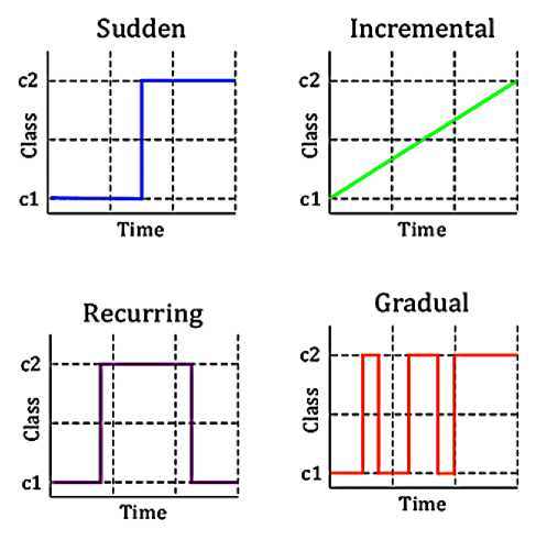
Fig. 1. Types of Concept Drift

This change can be an attribute change, a class conditional change or both. Further a concept drift can be sudden, gradual, recurring, or incremental drift as shown in Fig.1. Sudden drift is felt when the distribution changes suddenly from class c1 to class c2 in the next time step. The drift is said to be gradual when the old concept gradually moves in the direction of the new concept, creating intermediate concepts. Drifts are recurrent when an old concept re-occurs after some time. The drift is incremental if at any point in time the two consecutive concepts are almost the same, but the change in concept is observed over a longer time period.

In our work, we are evaluating the various online algorithms [28] which take as input a single labeled training instance as well as a hypothesis and output an updated hypothesis. For a given sequence of instances, an online algorithm will produce a sequence of hypotheses. The online approaches give more importance to stability when the concept is stable, and reduce classification errors while handling drifting data streams. These approaches always try to minimize the time and memory requirements for any system.

Further, the online approaches can be divided into approaches that use a mechanism to deal with concept drift [9, 11, 17, 18, 21]; and approaches that do not explicitly use a mechanism to detect drifts [12-14, 19, 36]. The former category of approaches such as early drift detection method (EDDM) [21] and Drift detection method (DDM) [9] use some measure related to the accuracy to handle drifts. They rebuild the system once a drift is detected / confirmed, and hence cannot be used to handle recurrent or predictable drifts. The latter set of approaches assigns weights to each base learner in the ensemble/ set of learners, as per its accuracy in predicting the class labels of new training instances e.g. Blum’s implementation of weighted majority (WM) [2,25] and Dynamic weighted majority (DWM) [12,14]. The ensemble of classifiers are continuously updated and trained by deletion of poor performing classifiers. These approaches give results that also accounts for earlier learning and experience. As these approaches, consider the old past, they can be easily used for recurrent or predictable drifts where almost no work has been done in the literature. Their classification results are highly reliable and accurate. It has been found that the success of an ensemble as in DDD [31] is based on the level of diversity between the classifiers. Diversity [32, 33, 34, 37] in an ensemble of classifiers measures the variation in the classification accuracy of ensemble members for a given training example. However, diversity cannot be treated as a replacement for the accuracy of the system.

In our work, we will evaluate EDDM, DDM, WM, DWM and the worst case learner i.e. standard implementation of naïve bayes (does not handle any drifts in concepts). For our study, we use the implementation of naïve bayes from Massive Online Analysis software tool [1]. We will also empirically present the influence of variation in the features of the various approaches, on their performance while handling drifting concepts. For the first time, these approaches would be compared in terms of new performance metrics such as kappa statistics, evaluation time and model-cost. Our paper is organized as follows. In the next section, we will be describing the new performance metrics used to evaluate the algorithms. In Section III, we will be giving a description of the various algorithms and in Section IV we will briefly describe the various artificial and real-world datasets that we will be using for the experimental evaluations. In Section V, the experimental results will be illustrated, discussed and compared in detail. In the last section, we will summarize our results and also discuss the scope for future research.

• II.    Description of the Performance metrics

Prequential accuracy (%): Prequential accuracy [3] is the average classification accuracy obtained by the prediction of an example to be learned prior to its learning, measured in an online way. This measure evaluates a classifier on a stream by testing then training with each example in sequence. It is computed using a sliding window along-with a fading factor forgetting mechanism. It is measured as percentage of correct predictions from total number of predictions made during testing [10].

Kappa statistic (%): The Kappa statistic value is a performance measure that gives a score of homogeneity among the experts. If experts are more homogeneous, they are likely to be less diverse and vice-versa. The level of diversity [7, 20] of a given set of experts that correctly classifies an instance depends upon the type of drift present in the given data stream.

Model cost (RAM-Hours): The resource efficiency of any stream mining algorithm is judged by another measure i.e. model-cost (RAM-Hours). One RAM-Hour is equivalent to one GB of RAM being deployed for one hour.

Evaluation Time (CPU-seconds): It is the average CPU runtime involved when testing of new instances and further training of classifiers based on data distributions underlying the training instances.

Memory (bytes): This measures the average amount of memory used by an algorithm. It can be divided into two categories: memory used to store the running statistics, and that used to store the online model.

• III.    Description of the Algorithms

• A.    Drift Detection Method (DDM)

DDM [9] monitors concept drifts in data streams based on the online error rate of the algorithm. When a new example arrives, it is classified using the current model. The method describes a warning level and a drift level. The approach is based on the fact that the error rate of the algorithm ( p i ) will reduce with each example if the concept is stationary. A significant increase in the error rate suggests that the concept is changing and the model needs to be rebuilt.

p_i + s_i ≥ p_min + 2. s_min                                 (2)

p_i + s_i ≥ p_min + 3. s_min                                  (3)

In (2) and (3) s i is the standard deviation, p min and s min are the p i and s i values, when p i + s i reached its minimum. The author defines two levels:

• •    a warning level as in (2), which predicts of a possible context change

• •    a drift level as in (3), at which drift is supposed to be true, the model is reset using examples stored since the warning level.

• B.    Early Drift Detection Method (EDDM)

EDDM [21] was developed to handle very slow gradual changes in data streams apart from handling gradual and abrupt drifts. EDDM explicitly handles drifts in dataset and is based on the estimated distance between two classification errors using two accuracy measures: average distance between two errors (pi) and the standard deviation (si). If this distance is large, this means the concept is stable and the new instances belong to the same earlier target concept. However, a small distance depicts changing concepts.

The author defines two levels:

• •    a warning level α (0<α<1), which predicts of a possible context change

• •    a drift level β (0<β<1), at which drift is supposed to be true and the model is reset using examples stored since the warning level.

If p and s keep on decreasing at every time step, the model would take minimum of 1/α time steps to reach the warning level and 1/β to reach the drift level. Hence, a model is kept for a minimum of 1/β time steps before it is reset.

• C.    Weighted Majority (WM)

Weighted Majority [2, 25] is an online approach based on the principle that a pair or a triplet of features is sufficient to get a good expert. Each expert makes predictions based on the values of their set of features. The final prediction (i.e. global prediction) is the weighted majority vote of all the ( ⁿ ₂ ) experts. Each expert is assigned an initial weight of one and if it predicts the class of the instance incorrectly, its weight is reduced by a multiplicative factor. A modification to WM is to remove the experts, whose weight drops to a given threshold value. This ensures that the algorithm speeds up with the progress in learning. WM approach was applicable only in situations where the experts were known a priori to learning, making it impractical for many real time data mining applications.

• D.    Dynamic Weighted Majority (DWM)

Dynamic Weighted Majority (DWM) [12, 14] is a modified version of WM. In addition to weight update of experts as per their predictive performance and removal of experts whose weight reach a given threshold value, DWM dynamically creates new experts when the final prediction is incorrect. A parameter p controls the creation, deletion or reduction in weight of the experts and helps DWM in dealing with drifts in case of large and noisy data sets. This has been proved in the experimental section of our paper. A variant of DWM defines a limit (m) on the maximum number of experts existing in the ensemble at any given time step. When the global prediction is incorrect and the number of experts reaches the size of the ensemble, a new expert is created only when the weakest expert having the minimum weight is removed from the ensemble.

• E.    The Naïve Bayes Classifier(NB)

The classifier performs Bayesian prediction while making a naive assumption that all inputs are independent. It is the simplest of all the algorithms with very low cost. We are using naïve bayes classifier that has been implemented in Massive Online Analysis software (MOA) [1]. Given nC different classes, the trained Naïve Bayes classifier predicts for every unlabelled instance the class C to which it belongs, with high accuracy. However, it has not been designed to handle any changes in concept and learns from all the examples in the data stream. Let there be k discrete attributes xi (1≤ i ≤ k), such that that xi can take ni different values. Let C be the class attribute which can take nC different values. On receiving an unlabelled instance I = (x1= v1, . . ., xk = vk ), the classifier computes the probability of the instance I being in class c, as in (4).

Pr [ C = c | I ] = ∏ i =1 ^k Pr [ x i = v i | C = c ] (4)

= Pr [C=c]. П i =i ^k Pr [ X i = V i ^л c = C ]/ Pr [ c = C ]

The values Pr [ x i = v i ^ C = c ] and Pr[ C = c ] as in (4), are estimated from the training examples. This algorithm is an incremental algorithm, that on receiving a new example (or a batch of new examples) increments the relevant counts.

• IV.    Concept Drifting Data Streams

• A.    Artificial Datasets

a Stagger Concepts: Abrupt concept drift without noise

A concept in a Stagger [15, 16] dataset consists of three attribute values: color ∈ {green, blue, red}, shape ∈ {triangle, circle, rectangle}, and size ∈ {small, medium, large}. The presentation of training examples lasts for 240 time steps, with one example at each time step. In this data set, we are evaluating a learner based on a maximum of a pair of features and in each context at least one of the features is irrelevant. In the first context (first 80 time steps), the examples having the concept description, size= small and color= red are classified as positive. In the next (80 time steps), the concept description is defined by two relevant attributes, color= green or shape= circle, and so size forms an irrelevant attribute .With the third context (next 80 time steps), the examples are classified as positive if size =medium or size = large. To evaluate the drift detection algorithm, we randomly generate 80 examples of the current target concept, and evaluate the learners’ prequential accuracy. In our experiments, we repeated this procedure 50 times and averaged the various parametric results over these runs.

b SEA Concepts: Very large dataset, abrupt concept drift with noise

y =[ x 0 + x 1 ≤ θ ],                                     (5)

where θ ∈{7, 8, 9, 9.5}one for each of the four data blocks. An example belongs to class 1 if condition in (5) is true and class 0 otherwise. Thus, only the first two attributes (x0, x1) are relevant and the third attribute is irrelevant. The presentation of training examples lasts for 50,000 time steps, with one example at each time step. For the first 12500 time steps, the target concept is with θ = 8. The second data block has θ = 9; the third data block has θ = 7; and the last concept has θ = 9.5. To evaluate the drift detection algorithm at each time step, we randomly generate 12500 examples of the current target concept, present these to the performance element and compute the prequential accuracy. We repeated this procedure 30 times and average the various measures over these 30 runs.

c Moving hyperplane: Gradual drift with noise

A hyperplane [8] in a d -dimensional space is the set of points x , x ∈ [0, 1], classified according to the constraint in (6) where x i is the i^th coordinate of x and a i , the weights of the moving hyperplane in each dimension i . Examples are labeled as positive, if it satisfies the condition in (6) else they are treated as negative. Threshold a 0 is calculated at each time step as in (7). The weights of the hyperplane initialized to [-1, 1] randomly, are updated at each time step as in (8), where t ∈ {-1, 1} is the change applied to every example and σ is the probability that the direction of change is reversed .

a0 ≤ Σi=1d ai xi(6)

a0 = ½ Σi=1d ai(7)

ai ^ ai + to(8)

Random noise was introduced by switching the labels of 5% of the training examples. The total number of examples in the data stream was 3000. At each time step, we presented each method with one example and computed its prequential accuracy. We repeated this procedure 30 times and the various parametric results are the average values over these 30 runs.

Table 1. List and type of attributes in Electricity pricing domain

Attribute                        Type day of week                                     Integer period of day                                       Integer the demand in New South Wales                 Numeric the demand in Victoria                           Numeric the amount of electricity scheduled for transfer between the two states                           Numeric

• B.    Real- World Datasets

a Electricity pricing domain

To evaluate our system on a real world problem, we selected the electricity pricing domain [22]. It was obtained from TransGrid, the electricity supplier in New South Wales, Australia. The dataset contains 45,312 instances collected at 30-minute intervals between 7May, 1996 and 5 December, 1998. Every instance in the dataset consists of five attributes listed as in Table 1 and a class label of either up or down.

The day of week and period of day contain integer values in [1, 7] and [1, 48], respectively. The remaining three attributes are numeric and measure the present demand: the demand in New South Wales, the demand in Victoria and the amount of electricity scheduled for transfer between the two states. The prediction task is to predict whether the price of electricity will go up or down and is affected by demand and supply.

b Breast Cancer dataset

The Breast Cancer dataset [5] taken from the UCI repository, classifies an instance as whether it belongs to the category of recurrence-events or no-recurrence-events based on 9 attribute values. This is one of three domains provided by the Oncology Institute that has repeatedly appeared in the machine learning literature. The data set includes total of 286 instances out of which 201 instances belong to one class and 85 instances belong to another class. Each instance is described by 9 attributes, having either linear values or nominal values.

• V.    Experimental Evaluation

In this section, we will provide a detailed description of the experimental results obtained after the evaluation of the approaches using various datasets discussed above.

The approaches which we will be evaluating are as under:

• 1.    A single expert approach that explicitly uses a mechanism to deal with drifts by monitoring the online error-rate of the algorithm i.e. DDM;

• 2.    A single expert approach that explicitly uses a mechanism to deal with drifts by monitoring the distances between two classification errors i.e. EDDM;

• 3.    An ensemble approach that does not explicitly use a mechanism to handle drifts and where the experts were known a priori to learning i.e. Blum’s implementation of WM;

• 4.    An ensemble approach that does not explicitly use a mechanism to handle drifts and dynamically creates or removes the experts in the ensemble i.e. DWM;

• 5.    Worst case learner i.e. standard implementation of naïve bayes.

Experiments were performed in MOA software [1], an open source framework for data stream mining applications. The various approaches were compared using the same base classifier naïve bayes (NB), so that the accuracy comparison is due to the concept drifting algorithms and not because of any variation in base classifiers.

We set the weighted-majority learners —DWM and WM with pairs of features as experts and the value of multiplicative factor β = 0.5. The threshold for removing the experts in weighted ensemble approaches was taken as 0.01 (i.e. θ = 0.01 in DWM and γ =0.01 in WM). For WM, each expert maintained a history of only its last prediction.

The values of the parameters: warning level ( α) and drift level ( β) in case of EDDM have been set to 0.95 and 0.90, respectively. The value of period p and the number of experts ( m ) varies in each dataset, so as to get optimum results for the weighted ensemble approaches. Our results provide the empirical support to the fact that the threshold value does have an impact on prequential accuracy and also on the other performance metrics. This directly challenges the earlier conclusion that the threshold value does not have any influence on accuracy. Another observation was that a change in the value of period ( p)

(the parameter that controlled the update to experts, creation and deletion of experts’ in DWM), had a great impact on the performance of DWM in terms of prequential accuracy.

(a)

(d)

(b)

(e)

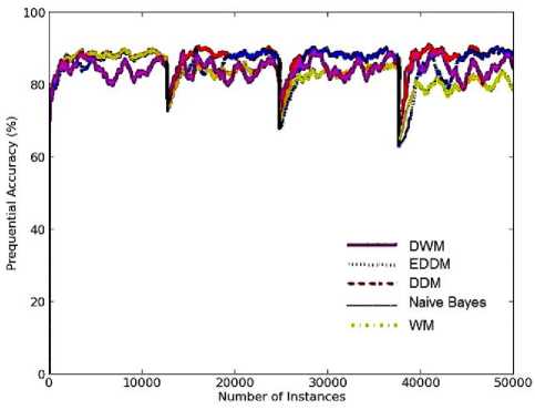
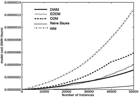
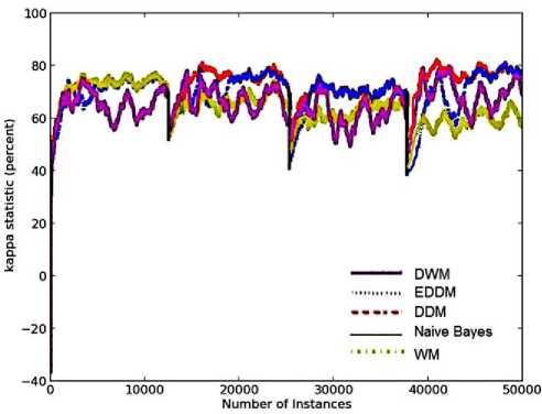
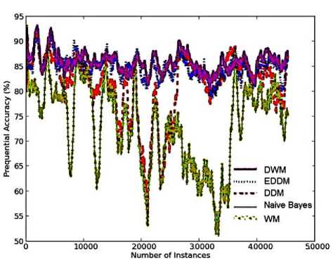
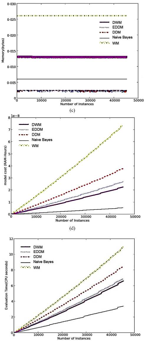
Fig. 2. Average results for the empirical evaluation of the various approaches on SEA dataset, containing 10% noise based on various performance parameters (a) Prequential accuracy (%) (b) kappa statistic (%) (c) Memory (bytes) (d) model cost (RAM-Hours) (e) Evaluation Time (CPU seconds)

О-020

О-015

£ 0-010

Number of Instances

(c)

Table 2. Average results of evaluation of DDM, EDDM, DWM, WM and naïve bayes (NB) on SEA Concepts, using naïve bayes as the base classifier

	DDM	EDDM	NB	WM	DWM
Prequential Accuracy	87.81	86.34	83.74	83.73	84.50
kappa statistic	72.90	69.85	64.70	64.5	65.64
model cost (*1e-7)	3.2	2.2	0.0	7.2	1.8
Evaluation Time	72.41	64.16	31.25	96.53	65.88
Memory	0.00	0.00	0.00	0.02	0.00

A. Comparison on SEA Concepts

To evaluate the various approaches, a new example was introduced at each time step and we computed the prequential accuracy averaged over 30 runs of the very large SEA dataset with 10% class noise. In case of weighted experts, the parameter p was set to 50 and maximum limit for the number of experts in the ensemble was set to 5.

DDM and EDDM gave very high prequential accuracies on all the four target concepts as illustrated in Fig.2(a). These approaches reset the model after the drift level is reached and a new model is learnt using the examples stored, since the warning level was triggered. Hence they do not have any memory of the earlier concepts, which is not even required in-case of sudden non-recurrent drifts in dataset.

On the first target concept, DWM performed the worst among all the approaches in terms of prequential accuracy as illustrated in Fig.2(a). However, with the progress in learning it illustrates higher accuracy levels similar as EDDM. DWM converged more quickly to the target concepts whereas EDDM reaches quite late, as seen on the fourth target concept with higher slope of DWM. This means, DWM maintains highly intelligent experts that adapt themselves quite early to the new concepts. But DWM has been found to detect changes in concept later than EDDM and DDM, as seen in the graph just before 37,500 time steps.

On the other three target concepts, Blum’s implementation of WM performed the worst as illustrated in Fig.2(a). WM approach does not have any mechanism to dynamically create new experts and trains the experts which are known apriori to learning. Naïve bayes performed similarly as WM, as seen by overlapping of their graphs on all the four target concepts. The standard implementation of naïve bayes performed the worst as it learns from all the examples in the stream, regardless of changes in the target concept.

DDM is shown to be more robust to noise as seen by its smooth curve in contrast to the fluctuating curves of the other approaches, as seen in Fig.2(a). On the other hand, DWM is highly sensitive to noise as seen by the higher rate of intense fluctuations in accuracy on all the four target concepts. It detects even a small change in distribution and improves its performance to reach accuracy levels as higher as EDDM. EDDM is more sensitive to noise than DDM, detects changes and improves its performance.

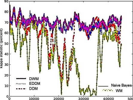
The kappa statistics describes the amount of homogeneity among the experts in the ensemble. Since DDM and EDDM are single expert models, they possess the maximum average value of kappa-statistic as can be seen in their graphs in Fig.2(b), on all the four target concepts. However, as EDDM is more sensitive to noise than DDM, its graph shows considerable number of fluctuations. With the progress in learning, WM and naïve bayes achieve lowest homogeneity among their experts as seen on the fourth target concept. However, DWM shows an improvement in the level of homogeneity with time. The graph for DWM is almost similar to that of DDM and better than EDDM and WM, in terms of slope as seen on the third and fourth target concepts. However, DWM shows the maximum variation in homogeneity levels among the experts on all the four target concepts. This is because of its high sensitivity to noise. Whenever there is an incorrect prediction in DWM, a new expert is created having a conceptual distribution different from the earlier concepts. This results in high diversity/ low homogeneity among its experts. However, with training of all the experts using the same training examples, the homogeneity among the experts’ increases and so the kappa statistic value.

As expected, Blum’s implementation of WM requires the maximum memory storage as illustrated in Fig.2(c ). It maintains large number of experts in the ensemble, each corresponding to a subset of features for any given training example.The memory consumption for WM is consistent throughout the process of predictions and learning as it trains fixed number of experts, which are known aprior to learning and no new experts are created. However, on the other hand DWM shows a sudden drop in memory requirements in the period surrounding 25,000 time steps. This is because of sudden drift at 25000 time steps, large number of experts gave incorrect predictions. This resulted in drop in their weights, reaching the given threshold value and removal of large number of experts from the ensemble. However, when the global prediction was incorrect, a new expert learned as per the new concept was created stabilizing the memory needs of DWM further. A small variation in memory requirements of DWM is because of presence of noise present in the dataset leading to updates, creation of new experts and removal of poor performing experts. DDM and EDDM required similar and the least memory requirements because they maintain a single expert in their models rather than an ensemble of experts as in DWM and WM. The memory needs of naïve bayes classifier is slightly more than EDDM and DDM.

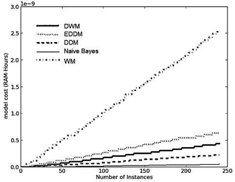
As explained earlier, the model cost tells us about the resource efficiency of any stream mining algorithm and for handling the data streams, this is a very mandatory requirement. Model cost is indirectly proportional to resource efficiency of any system. Compared to all the other approaches, as WM maintains the maximum number of experts in its ensemble, it requires maximum RAM-Hours to train these experts and is the least resource efficient. The graphs for all the systems show an exponential rise in model-cost with each time step, as illustrated in Fig.2(d). DDM also shows exponenetial trend as WM but after sufficient learning of the model around time steps 37500, the error rate reduces leading to a decrease in the slope of the graph. DWM requires more RAM-Hours than EDDM on the first and second target concepts. However, when its memory needs suddenly dropped at 25000 time steps as seen in Fig.2(c ), the resource efficiency of DWM improved and turned out to be better than EDDM. DDM requires more RAM-Hours than EDDM at every time step and is found to be is less resource effective than EDDM. Naïve bayes has been found to be the most efficient among all the approaches in terms of RAM-Hours but it does not have any mechanism to cope with concept drift, giving very low accuracy levels.

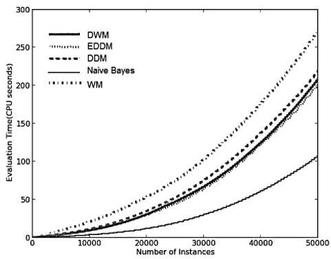
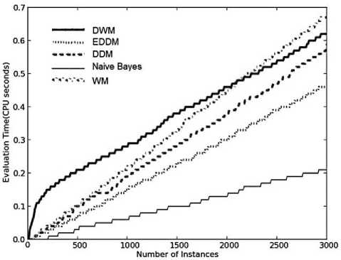
As illustrated in Fig.2(e), the evaluation time graphs for all the approaches show an exponential rise in CPU time, required to evaluate the systems, at each time step.

WM requires the maximum CPU time as it trains and updates maximum number of experts at each time step.

Naïve bayes requires least time as it does not updates the experts as per change in concepts, so least CPU involvement. The graphs for DWM and EDDM are similar in terms of slope and asymptote as seen by overlapping of their curves at each time step. EDDM is found to be better than DDM in terms of average CPU involvement, making EDDM more time efficient. Table 2 provides us with the average experimental results for the various approaches on the SEA concepts with 10% class noise. This was the first time that the kappa-statistic values, the model-cost, the CPU evaluation time and the memory usage of these algorithms have been discussed.

(a)

(b)

(c )

(d)

(e)

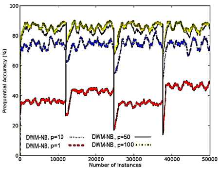
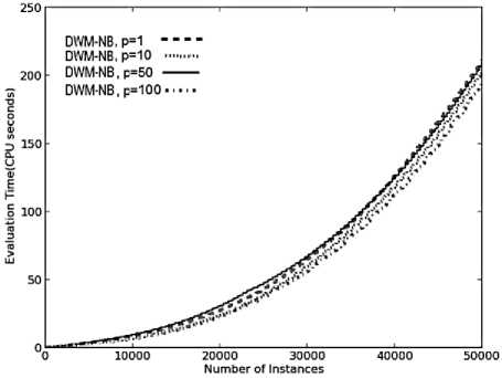
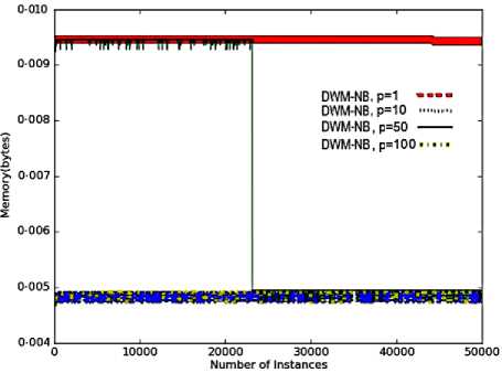
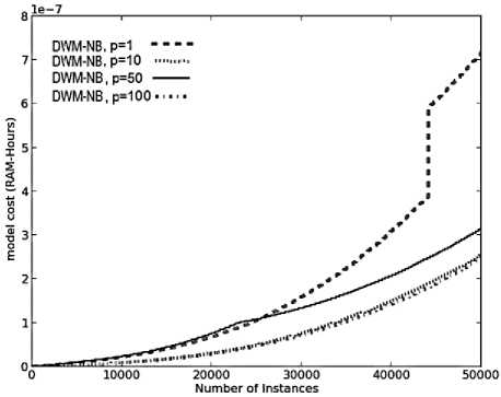
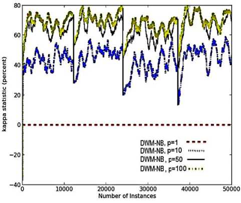
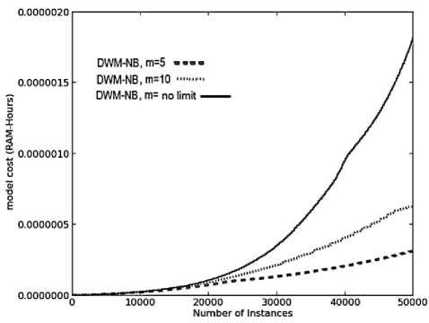
Fig. 3. Average results for empirical evaluation of DWM on SEA Concepts with the variation in period ( p) value placing a limit on the number of experts to 5, based on various performance parameters (a) Prequential accuracy (%) (b) Evaluation time (CPU seconds) (c) Memory (bytes) (d) model cost (RAM-Hours) (e) kappa statistic (%)

(a)

(b)

(e)

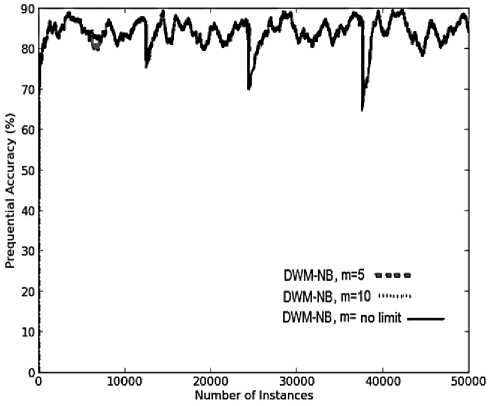
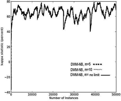
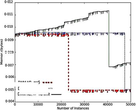
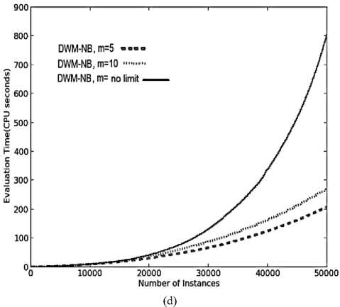
Fig. 4. Average results for empirical evaluation of DWM on SEA Concepts with the variation in number of experts (m ) value keeping period value of 50, based on various performance parameters (a) Prequential accuracy (%) (b) kappa statistic (%) (c) Memory (bytes) (d) Evaluation time (CPU seconds) (e) model cost (RAM-Hours).

>■ 0008

DWM-NB,m=5

DWM-NB,m=10 .......

DWM-NB, m= no limit

(c)

A comparison of EDDM and DDM, led us to the conclusion that EDDM is a better approach than DDM in handling noisy datasets containing sudden drifts. This is because EDDM achieves almost similar average prequential accuracy as DDM, within lesser time and lower model cost. Comparing WM and DWM, with the progress in learning DWM achieves better prequential accuracy than WM, in lesser time and memory requirements so resulting in a more resource effective system. Naïve bayes is a good base classifier when the system is without any drifts but in a dynamically changing system, the results are not very accurate. Based on all the above experimental evaluations, EDDM and DWM are very good candidates for handling very large noisy datasets containing abrupt drift.

The impact of variation in the period (p) value on the performance metrics

The period ( p ) tells us how often DWM updates, creates or removes the experts. In noisy domains, a small period value ( p set to 1) increases the rate of update to experts which give incorrect predictions as illustrated in Fig.3(a). These experts would be removed very early from the ensemble such that they do not get enough time for learning. This would further increase the number of incorrect global predictions, leading to an increase in the rate of creation of new experts seen as a thick line in Fig.3(c ), for p value of 1. Thus, the lack of training of experts results in minimum prequential accuracy for DWM as illustrated in Fig.3(a). However, when sudden drift is detected by the system, it converges more quickly to the new target concepts when p is set to 1, than it did with higher values of p. This is because the system with p set to 1, creates a new expert trained on the new concept within next time step .

The kappa-statistic value for DWM with p value of 1, becomes zero as a new expert is highly different in concept from the earlier experts (which got hardly no time for training), giving zero level of homogeneity among the experts as seen in Fig.3(e). However, with the increase in the value of period, experts got more time for training on the training instances, increasing their level of homogeneity and handling noise in dataset. Hence, prequential accuracy and kappa-statistic metrics in case of noisy sudden drifting domains are directly proportional to the period value as seen in Fig.3(a) and 3(e).

However, these obervations are not true for the other performance metrics. A system with p value set to 1, has an increased frequency of updates , creation and removal of experts resulting in an increase in the overall evaluation time, memory requirements and model-cost as illustrated in Fig.3(b), 3(c) and 3(d) respectively. When p value is set to 10, there is a decrease in the rate of updates, creation and removal of experts as experts (giving incorrect predictions) could be updated only after 10 time steps , resulting in lower CPU evaluation time, memory requirements and RAM-Hours. However, in a system with p set to 50, the updates to poor performing experts could be made only after every 50 time steps. The rate of removal of experts was also reduced as the experts’ weight took more time to reach the threshold value. As a result, these experts got enough time for training so as to adapt themselves to the new concept resulting in more evaluation time, more memory to store large number of experts and increased model cost, than the system with p value of 10. The memory requirements in this system dropped suddenly at 25,000 time steps as illustrated in Fig.3(c). The graph depicts that large number of poor performing experts were removed from the system, whose weights reached the threshold value within last 50 time steps.

When p was set to 100, the rate of updates was reduced further, reducing the rate of removal of experts, reducing the average time (required to update the experts) and reducing the cost of the system (almost equivalent to that needed by the DWM system with p set to 10). By analysing the results presented in Fig.3, we can easily conclude that the CPU evaluation time and the cost involved is directly proportional to the number of experts ( i.e. memory requirements), existing at any given time step. Hence, the parameter p is necessary and really useful for large noisy datasets, as can be seen with the system with p value set to 100. This system has a very high prequential accuracy and kappa-statistic with reduced evaluation time and memory requirements, giving a highly resource effective system.

The impact of variation in the number of experts (m) on the performance metrics

In DWM, the variation in the number of experts does not impact the performance in terms of prequential accuracy and kappa statistics as seen by overlapping of the graphs for various values of m ( maximum limit on the number of experts) as seen in Fig.4(a) and 4(b), respectively. However, it does impact the average evaluation time , the memory requirements and the resource effectiveness of the system.

The number of experts itself explains that DWM with no limit on the number of experts maintained maximum number of experts at any given time step and hence the system has the maximum memory requirements. Further, m value of 5 has lower memory needs than the system with m value of 10 experts as seen in Fig.4(c ). The sudden fall in memory requirements of all the systems is because of the period value of 50 and not because of any other parameter. As the number of experts existing in the ensemble increases, the average evaluation time required to update the experts increases’ exponentially and correspondingly the cost of the system also increases as seen in Fig.4(d) and 4(e) respectively, without any improvement in the prequential accuracy. Hence, it is always better to limit the number of experts so as to get the best reults even in a resource constrained environment.

From analysis of the experimental results, DWM and EDDM are highly competitive in handling concept drifts in SEA dataset. EDDM is more robust to noise than DWM. Both the approaches have almost similar CPU involvement and model cost. However, DWM requires more memory than EDDM as it maintains an ensemble of experts describing concepts varying from previous target concepts to the new target concepts, wheras EDDM contains a single expert learned from examples stored since the warning level was triggered and does not account for earlier learning and experience. Hence, DWM is the best candidate for handling abrupt drift in a very large dataset containing noise. Another conclusion is that the period value greatly helps in large and noisy domains, by achieving very high accuracies within reduced time and memory requirements. Further, the lower the value of number of experts existing in an ensemble at any given time step, lower is the memory requirements and lower is the model cost without any loss in accuracy even in noisy domains.

• B.    Comparison on Stagger Concepts

To evaluate the drift detection algorithm DWM on Stagger concepts, we set it to update experts’ weights and create or remove experts every ten time steps (i.e. p = 10). The maximum limit for the number of experts in the ensemble is set to 10.

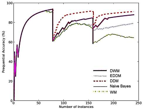
On the first target concept, all the approaches show similar performance in terms of prequential accuracy as seen by overlapping of their graphs in Fig.5 (a). However, DDM performs the best giving maximum accuracy on the second and third target concepts. It converges quickly to the target concepts achieving higher accuracy levels. Naïve bayes performed the worst as it does not have any direct provision to remove outdated concept descriptions. Blum’s implementation of WM performed similar as naïve bayes i.e. the worst case learner on the second and third target concepts. Both these approaches detected false alarms on the first and second target concepts as seen in the period surrounding time steps, 80 and 160 in Fig. 5(a).

EDDM performs similarly as WM on the second target concepts giving very poor prequential accuracy while it achieved better accuracy than WM approach, on the third target concept. DWM performs better than EDDM and WM on the second and third target concepts in terms of prequential accuracy giving higher slope, converging more quickly to the target concepts. This proves that DWM is a very good candidate to handle sudden drifts in dataset with or without noise.

(a)

(d)

(b)

(e)

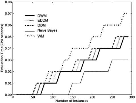
Fig. 5. Average results for empirical evaluation of the various approaches using Stagger Concepts based on various performance parameters (a) Prequential accuracy (%) (b) kappa statistic (%) (c) Memory (bytes) (d) model cost (RAM-Hours) (e) Evaluation Time (CPU seconds)

(c)

Table 3. Average results of evaluation of EDDM, DDM, naïve bayes, WM and DWM on Stagger Concepts

	DDM	EDDM	NB	WM	DWM
Prequential accuracy	86.50	79.16	76.04	76.03	83.32
kappa statistic	74.32	59.58	53.37	53.37	67.89
model cost (*1e-9)	0.25	0.35	0.04	1.25	0.31
Evaluation Time	0.07	0.11	0.03	0.21	0.09
Memory	0.00	0.00	0.00	0.02	0.01

EDDM detects non-accurate drifts as can be inferred from the accuracy curves of EDDM which shows a slight negative slope whereas the graphs of DWM and DDM, show an increasing trend as in Fig. 5(a). So from analysis of the results on SEA concepts and Stagger concepts, DDM achieved very high accuracy levels on datasets containing abrupt drift irrespective of noise present in the dataset. It can be seen that in the absence of noise (i.e. Stagger concepts), the curves are very smooth in nature and have reduced rate of fluctuations in accuracy levels.

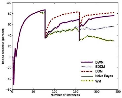
The level of homogeneity is the same for all the approaches on the first target concept as seen in Fig.5 (b). However on the second and third target concepts, DDM gives the best homogeneity as it maintains only a single expert, which is reset when drift level is reached and a new model is learnt using examples (that all nearly belong to the same concept) stored since the warning level. On the second and third target concepts, WM and naïve bayes showed the minimum level of homogeneity among its experts. This is because naïve bayes does not have provisions to remove the outdated concept descriptions.

DWM gave better trained experts with higher level of homogeneity, better than EDDM on second and third target concepts as illustrated in Fig. 5(b). The graphs for kappa statistic show similar trend as accuracy graphs corresponding to each approach. This is because when concept drift occurs, the accuracy in classifying the new examples drops, leading to deletion of experts as in DWM. When the global prediction is incorrect, a new expert based on the new concept is created that is different from the earlier concepts resulting in drop in the homogeneity among the experts. With the progress in learning, all the experts are trained as per the new concept. This results in an increase in similarity among the experts, resulting in improvement in accuracy levels as seen in the period just after time steps 80 and 160. EDDM, WM and naïve bayes depict higher variation among the experts on the second target concepts. However, on the third target concept EDDM shows an increase in its homogeneity levels.

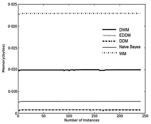
WM requires the maximum storage for its ensemble as explained earlier in the experimental evaluation using SEA concepts. However, when noise is not present in the dataset, DWM shows almost consistent memory needs like the other online approaches as seen in Fig.5(c). This is in contrast to its behavior on SEA concepts as seen in the last section. This is because when noise was present in the dataset, large number of misclassifications resulted in large number of weight updates of experts, reaching the weights below threshold value, and resulting in removal of large number of experts. However, when noise was not present the updates to experts and removal of experts happened only when drifts occurred in datasets. This increased the average memory needs of DWM. DDM and EDDM required least storage as they maintain a single expert whereas naïve bayes required almost double the storage as needed by EDDM approach. Hence, we can conclude that the relative memory requirements of each of these approaches, is dependent on the methodology underlying the approach, irrespective of the dataset used for evaluation.

The graphs for model cost are linear for all the approaches when the dataset does not contain noise as seen in Fig.5 (d). However, when noise was present in the dataset these graphs depicted an exponential trend as seen in last section. This means the presence of noise increased the cost of each of the systems at each time step. This is because of higher rate of updates to experts, and removal of poor performing experts in noisy domains.

In case of Stagger concepts, WM is the most costly model as it maintains trains and updates large number of experts as seen in Fig.5 (d). Naïve bayes is the least costly approach as explained earlier. DDM was better than EDDM and DWM with their graph having a lower slope, hence DDM was highly resource effective than the other two approaches. This is because the absence of noise lowers the error rate, reduces the frequency of model reset and learning of new models. Similarly, DWM proved to be less costly than EDDM because of reduced rate of expert updates, creation of new experts and removal of poor performing experts in DWM when noise was not present in dataset.

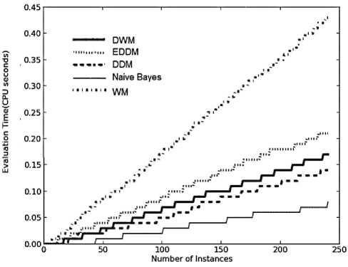
As illustrated in Fig. 5(e), all the approaches show a linear rise in evaluation time while handling drifts in Stagger concepts, whereas they show an exponential rise in the presence of noise as illustrated in Fig. 2(e). When noise was present, rate of updates and removal of experts was higher. This involved more CPU time and hence the graphs for SEA concepts were exponential in nature. However when no noise was present, the number of updates to experts, creation and removal of experts dropped considerably giving a linear rise in evaluation time. WM requires maximum CPU involvement whereas naïve bayes requires least CPU time.

EDDM needs more CPU time than DWM, followed by DDM which proves to be the best approach for Stagger concepts. DDM gave very high accuracies in real time and memory and proves to be the best resource effective system. The experimental results averaged over 50 runs of Stagger concepts have been tabulated as in Table 3.

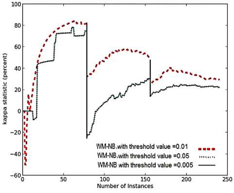
Impact of variation in threshold value and the multiplicative factor in weighted majority algorithm

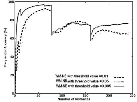
The variation in the value of threshold, greatly affects the performance of Blum’s implementation of weighted majoritry as seen in the experimetal evaluation using Stagger concepts (containing abrupt drift without noise). We performed experimental evaluations by varying the threshold value between 0.01, 0.05 or 0.005, keeping the value of multiplicative factor to be 0.5.

(a)

(b)

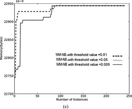
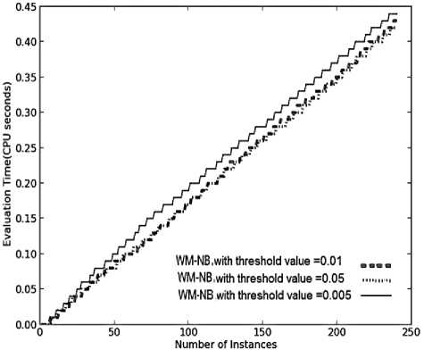
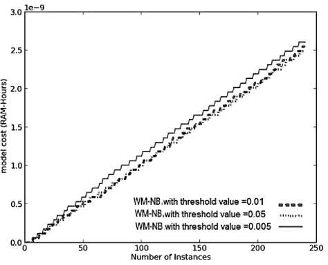
Fig. 6. Average results for empirical evaluation of WM approach on Stagger concepts using different values of threshold, keeping the multiplicative factor to be 0.5 based on various performance parameters (a) Prequential accuracy(%) (b) Evaluation time (CPU seconds) (c) model cost (RAM-Hours) (d) kappa statistic (%) (e) Memory (bytes)

(c)

Table. 4. results of evaluation of WM with different values of multiplicative factor ( β ) keeping threshold value of 0.01, on Stagger concepts

	WM with β =0.5	WM with β =0.9
Prequential accuracy	76.03	76.03
Kappa statistic	53.37	53.37
model cost (*1e-9)	1.25	1.25
Evaluation	0.21	0.21
Time
Memory	0.02	0.02

(d)

As seen in Fig.6 (a), decreasing the threshold from 0.01 to 0.005, improves the prequential accuracy. The drop in threshold means, experts were allowed to remain in the ensemble for a longer time duration, giving more time to train the experts. As seen on the second and third target concepts, the system with threshold value of 0.005 was better than the system with threshold value of 0.01 in terms of slope. It converged more quickly, reaching higher accuracies to the target concepts.

Similar performance was observed for WM with threshold value of 0.005 and 0.05, in terms of prequential accuracy. In this case larger value of threshold (i.e. 0.05), results in removal of poor performing experts at an earlier stage. This helps in maintaining only good performing experts, giving accuracy as high as system with threshold value of 0.005, that too within lesser time and model cost as seen in Fig.6 (a), 6(b) and 6(c), respectively. This system with θ =0.05, maintains only good performing experts, so the time required to update these experts is quite low, providing a system which is highly resource effective.

As even the poor performing experts in the WM sytem with threshold of 0.005, were trained and updated for a longer time duration, the total evaluation time and the model cost was higher than that needed by weighted majority systems with threshold value of 0.01 and 0.05, as seen in Fig.6 (b) and 6(c), respectively. It has been observed in Fig.6 (d) and 6(a), that WM with threshold of 0.01, gave the highest average value of kappa statistic on all the three target concepts and gave worst average prequential accuracy in classifying the new instances. This proves that a highly diversified ensemble provides better accuracy than a more homogeneous ensemble in classifying the instances that contain sudden drifts in concept.

As illustrated in Fig.6(e), the average memory requirements of WM algorithm with different values of threshold, were the same on the second and third target concepts. However, on the first target concept, WM with threshold of 0.05 and 0.005 maintained lesser number of experts than WM with threshold of 0.01. Hence, the best system is WM with threshold of 0.05 achieiving very high accuracy in real time and memory, giving a highly resource effective system.

The variation in the multiplicative factor, β does not impact the performance of WM system in terms of any performance metrics. Experimental results were performed with WM using, 0.9 and 0.5 as the multiplicative factor. Both the systems showed similar performance giving similar accuracy; similar level of homogeneity; similar memory requirements i.e. both these sysyems maintained similar number of experts at every single time step; and classified all the instances within same average evaluation time with same resource utilization. Hence varying the multiplicative factor, does not bring any significant change in the performance of WM algorithm. The results for both these systems over the different performance metrics are the same as seen in Table 4.

• C.    Comparison on hyperplane dataset

  The online learning system was tested with 10% examples generated randomly according to the given concept and trained with the rest 90% training examples. The total number of dataset instances used for evaluating the systems was 3000, with every new instance at each time step. Noise was introduced in the dataset by switching the class labels of 5% of the examples. The best results for the various parameters were achieved by setting the following values: the number of dimensions i.e. d = 10, magnitude of change is 0 . 001 i.e. t=0.001, number of drifting attributes is 10, and the number of class labels is 5. DWM showed best accuracy when the parameter p was set to fifty time steps (i.e., p = 50). The maximum limit for the number of experts in the ensemble was set to 4. The value of σ was set to 10. Sudden and significant changes were introduced every 1000 time steps.

As observed from the graphs in Fig.7 (a), before 1000 time steps DWM, WM and DDM performed similarly in terms of prequential accuracy on the moving hyperplane dataset containing gradual drifts in concept. EDDM performed the worst on the first target concept. However, the graphs for the approaches are similar in terms of slope and asymptote. After 1000 time steps, with the progress in learning the distance between two classification errors increases, such that EDDM achieves higher accuracies as

DDM, naïve bayes and WM approach. This is because EDDM is very sensitive to noise present in the dataset, detects changes and improves its performance.

DWM and Blum’s implementation of WM perform similarly until the accuracy of DWM gradually drops in the period surrounding time steps 1300. This is because when a gradual noisy drift occurs, DWM gradually updates its experts to adapt to the new concept but as DWM is highly sensitive to noise, large numbers of misclassifications happen, resulting in removal of large number of highly trained experts and drop in prequential accuracy.

Simple naïve bayes classifier achieves very high accuracies on all the three target concepts even if it is not designed to handle drifts in data. WM performed better than EDDM in terms of accuracy as seen in the period surrounding time step 1500 when handling gradual drifts, and converged more quickly to the target concepts than EDDM. In the period surrounding 2000 time steps, with the extensive training and relearning of the EDDM model, it achieves accuracies as high as WM approach as seen by overlapping of their graphs. After 2000 time steps, DWM achieves the least accuracy levels among all the online systems. Hence, for datasets containing gradual drifts and noise, DWM is highly incompetent approach for handling drifts in data.

The relative behavior of various approaches in terms of kappa-statistic is similar as their behavior in terms of prequential accuracy. All the approaches maintained experts which were highly homogeneous in concept, apart from DWM that achieves very high diversity among its experts. This is so because the weight of the experts in DWM are updated frequently because of noise and gradual drifts present in the dataset ultimately leading to removal of large number of experts whose weight reaches the threshold value. When global prediction was wrong a new expert learned on the new concept was created.

This was controlled by the period value, which created the new expert which was quite different from the experts already existing in the dataset (gradually drifting dataset results in large variation in concept after every p time steps).

(a)

(b)

(c)

(d)

Fig. 7. Average results for empirical evaluation of various approaches on hyperplane dataset with gradual changes and 5% noise, based on various performance parameters (a) Prequential accuracy (%) (b) Memory (bytes) (c) model cost (RAM-Hours) (d) Evaluation time (CPU seconds)

WM requires the maximum memory whereas DDM and EDDM requires the minimum memory among all the other approaches for their evaluation, independent of the type of dataset as seen in Fig.2(c), 5(c) and 7(b). However, in moving hyperplane problem the memory required by each of the approaches has increased by a considerable value as compared to the earlier requirements on SEA and Stagger concepts, but they are almost consistent at each time step.

The memory requirements for DWM, is almost four times the requirements of EDDM and DDM. This is because in DWM we have set the maximum size of ensemble to be 4 experts that happens to be four times the size of a single expert model such as EDDM and DDM. WM would not be a good online approach to handle gradual conceptual changes in online data, owing to its maximum storage needs irrespective of its higher accuracy levels as seen in Fig.7 (b) and Fig. 7(a), respectively. The model cost graphs for the various approaches observe a linear rise in the demand for RAMHours as seen in Fig.7(c). As expected, WM has the highest demand for RAM-Hours and naïve bayes has the minimum demand among the various approaches. DWM needed more RAM-Hours than DDM and EDDM.

However, after 2100 time steps DWM’s demand for RAM-Hours reduces to the level of EDDM. On an average, DDM requires more RAM-Hours than EDDM; hence it is a less resource effective approach. So, comparing DDM and EDDM based on the parameter RAM-Hours, EDDM proves to be a more efficient real time approach achieving accuracies similar as DDM.

(a)

Number of Instances

(b)

(e)

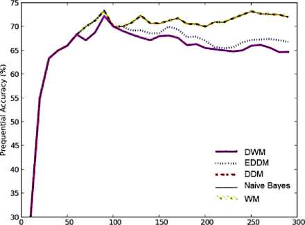
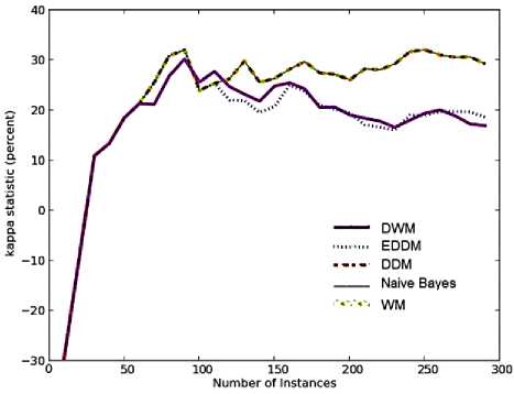
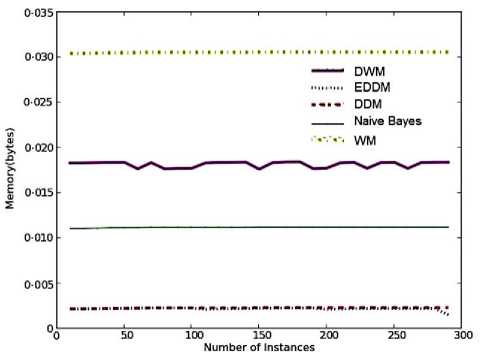
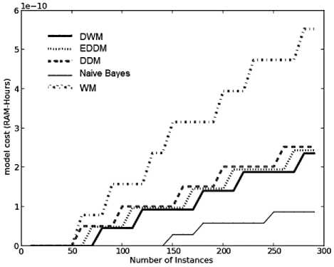
Fig. 8. Average results for empirical evaluation of various approaches on Electricity pricing dataset based on various performance parameters

(a) Prequential Accuracy (%) (b) kappa statistic (%) (c) Memory (bytes) (d) model cost (RAM-Hours) (e) Evaluation time (CPU seconds)

DWM needs maximum CPU involvement when evaluated on moving hyperplane problem, even more than that needed by WM as seen in Fig.7 (d), as gradual drifts and noise present in the dataset results in very high frequency of expert updates, removal and creation of new experts. However, after 2100 time steps the CPU time requirements reduces to a level which is even lower than that of WM. EDDM is better than DDM as seen from their graphs, as the graph for EDDM has a lower slope than that of DDM. As expected, naïve bayes requires the least CPU time. However, even though naïve bayes has not been designed to handle concept drifts in data, the learner achieves very high accuracy as extensive training of the classifier itself helps in handling gradual changes in the dataset. Table 5 gives the experimental results averaged over 30 runs of the hyperplane dataset. All the approaches are highly resource effective as seen by the value of the parameter RAM-Hours.

Table 5. Average results for evaluation of the concept drifting approaches on moving hyperplane dataset

	DDM	EDDM	NB	WM	DWM
Prequential accuracy	86.69	85.31	86.68	86.68	83.44
kappa statistic	73.24	70.46	73.23	73.23	66.74
model cost (*1e-9)	1.15	1.05	0.20	2.25	1.16
Evaluation Time	0.29	0.23	0.10	0.33	0.34
Memory	0.00	0.00	0.01	0.03	0.01

This is the first time that DWM and EDDM have been implemented on the rotating hyperplane problem. This was the first time that the kappa-statistic values, the evaluation time and the memory usage of these algorithms have been discussed on hyperplane dataset. From the analysis of the results, we can easily state that EDDM is the best online concept drift approach to handle gradual changes in a noisy domain. The standard implementation of naïve bayes, proved it to be a very good learner even if it was not designed to handle any kind of concept drift in dataset.

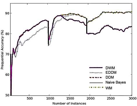
• D.    Comparison on Electricity pricing dataset

Since the Electricity pricing dataset is online, we processed the examples in the order they appeared in the dataset. We first obtained predictions using each example in the test set and then performed learning using the example. The period value for DWM has been set to 10 and the maximum ensemble size is 15. As this dataset is a real world dataset we cannot know exactly if or when the drifts occurred. However, experimental evaluations of the various sytems on this dataset provide us a comparative performance of each of the systems.

As predicting the price of electricity is an online task, we processed the examples in temporal order i.e. the order they appeared in the dataset. DWM has been found to be very robust to change as compared to the other approaches. This can be observed in Fig.8(a), around time steps 10,000 where the accuracy for DWM has been found to be nearly consistent, whereas WM, DDM and naïve bayes show large fluctuations in their accuracies during this period. Most illustrative is sudden drop of nearly 30% in accuracy of WM, naïve bayes and DDM whereas the accuracy for DWM and EDDM showed nearly 5% drop, between time steps 19,000 and 21,000. EDDM converges more quickly to the target concepts than DWM, however DWM provides better accuracy than EDDM. This is easily visible in the graphs at time steps, 22,000 and 27,500.

Table 6. Average results of evaluation of various approaches on real time Electricity pricing dataset

	DDM	EDDM	NB	WM	DWM
Prequential accuracy	81.15	84.82	73.41	73.41	85.86
kappa statistic	59.98	68.38	39.96	39.96	70.68
model cost (* 1e-8)	1.95	1.41	0.25	3.75	1.12
Evaluation Time	4.06	3.29	1.60	5.25	3.10
Memory	0.00	0.00	0.01	0.02	0.01

With the progress in learning, DDM achieves higher accuracies as EDDM and DWM, as is visible in the figure after time steps 27,000. Hence in terms of accuracy measure, the appropriate candidates for this domain are DWM and EDDM, with average accuracy of 85.86% and 84.82% respectively as listed in Table 6.

The experts in case of WM vary from being highly homogeneous to highly diverse over a fraction of small number of instances as can be seen in Fig.8(b), between time steps, 19,000 and 21,000 with drop of nearly 67% in kappa-statistic measure over a period of 2000 time steps. On the other hand, DWM and EDDM maintain experts which are highly homogeneous with their kappa-statistic ranging from maximum value of 85% to minimum value of 60%, over the complete domain of 45,312 instances.

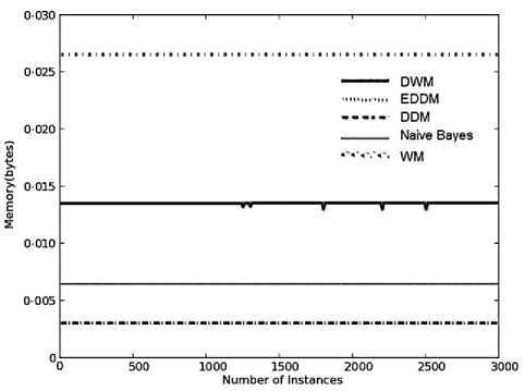
The memory requirements of the various approaches on electricity pricing domain, are almost consistent like the experimental evaluations on various datasets described earlier in our work as seen in Fig.8(c). The relative positioning of the various memory graphs, each corresponding to an online approach, depends only on the online approach selected for handling drifts, and is independent of the type and size of dataset, the type of drift, presence or absence of noise in the dataset. i.e. WM has the highest memory utilization followed by DWM approach, followed by naïve bayes and the least requirements are that of DDM and EDDM, each being a single expert model.

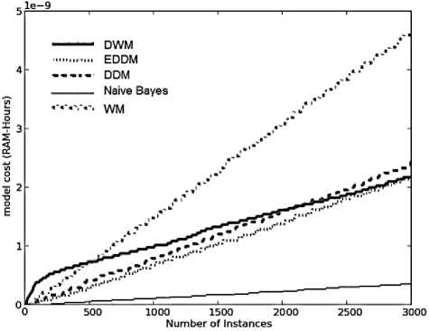
WM is the most costly model and requires the maximum CPU processing time as seen in Fig.8(d) and 8(e), respectively as WM maintains large number of experts at all time steps which are continuously updated as per their classification performance. On the other hand, naïve bayes is highly resource effective and requires the least CPU utilization as it does not have to maintain and update an ensemble of large number of experts as per any type of drift. The model-cost and time graphs for DDM has a higher slope than EDDM as seen in Fig.8(d) and 8(e), respectively. This is because DDM is more sensitive to changes in concept (as seen in Fig.8(a) by DDM’s accuracy graph) and rate of updates are higher than EDDM, involving more CPU time and more resource utilization. Similar is the observation for DWM and EDDM. DWM ( an ensemble of experts) is more resource efficient requiring lower number of RAM-Hours and lower CPU involvement than EDDM (which is a single expert model), at any given time step. This supports the claim that DWM presents a more stable system than EDDM. Hence based on the accuracy measure, model-cost, and average evaluation time, we can easily state that DWM is the best candidate for handling changes in the Electricity pricing real time dataset. The experimental results for all these approaches using Electricity pricing dataset have been tabulated as in Table 6.

Number of Instances

(a)

(b)

(c)

(d)

(e)

Fig. 9. Average results for empirical evaluation of the concept drifting approaches on Breast Cancer dataset based on various performance parameters (a) Prequential Accuracy (%) (b) kappa statistic (%) (c) Memory (bytes) (d) model cost (RAM-Hours) (e) Evaluation Time (CPU seconds)

Table 7. Average results for evaluation of the concept drifting approaches on Breast cancer dataset

	DDM	EDDM	NB	WM	DWM
Prequential accuracy	68.62	66.18	68.62	68.62	65.06
Kappa statistic	26.11	20.67	26.11	26.11	20.75
model cost (*1e-10)	1.32	1.20	0.43	2.72	1.14
Evaluation Time	0.02	0.02	0.01	0.03	0.02
Memory	0.00	0.00	0.01	0.03	0.02

• E.    Comparison on Breast cancer dataset

Another real time dataset that was used to empirically compare the above approaches was Breast Cancer dataset from the UCI Repository [5]. 10% of the examples were used as a testing set and the remaining 90% were used for training of the learners. Prequential accuracy of the various approaches was calculated over each instance, one instance at each time step, until all the instances in the dataset have been processed. This procedure for first testing and then learning using examples in the dataset was repeated over a one week period and the results were the average performance results for all these observations. The updates, creation and removal of experts in DWM can occur only after intervals of 10 time steps and the ensemble approaches can maintain maximum of 5 experts at any time step.

As Breast Cancer dataset is a real world problem, we are not sure when drifts occur and if they occur or not. It has been observed from the graphs in Fig.9 (a), in the initial time steps all the approaches perform similarly in terms of prequential accuracy. However, with extensive training of the experts all these online approaches gradually achieved very high accuracies, nearly 74% as seen as a peak at time steps 90. At time steps 60, when there is an incorrect prediction, DWM removes experts which have weights below threshold value, thus gradually reducing its memory requirements as seen in Fig.9(c). When global prediction is incorrect, DWM creates a new expert increasing its memory requirements and trains all the experts in the ensemble, resulting in a very quick improvement in its accuracy.

Around the period surrounding time steps 110, EDDM’s and DWM’s accuracy levels drop showing a negative slope whereas the other approaches ( WM, naïve bayes and DDM) show an exponential rise in their accuracies. On an average, EDDM achieve higher accuracies than DWM, with an average differential of nearly 1.12%. DWM gives us a more stable system than EDDM. This is illustrative in Fig.9 (a) during the period between time steps 160 and 210, where EDDM’s accuracy drops by nearly 5% whereas DWM’s accuracy drops by nearly 2.5 %. WM and DDM show almost constant accuracy during this time period, giving us highly stable systems. Hence in terms of prequential accuracy, WM and DDM provide us with very good predictions whereas DWM performs very badly resulting in lowest average accuracy values.

On an average, weighted majority maintains highly homogeneous experts as seen in Fig.9 (b). This is because it does not have the mechanism to dynamically create new experts as in DWM and only trains the existing set of experts known a-priori to learning, so the chances of highly diversified experts in WM is almost zero.

DDM has similar value of kappa statistic as EDDM at each time step, maintaining a single expert in their systems. This can be seen as their graphs overlap at every single time step until 110 time steps. However, in the period surrounding 110 time steps when the accuracy of EDDM drops, a new model is learnt using the examples stored since the warning level was triggered. This reduced the level of homogeneity in the EDDM approach. DWM maintains experts that are less homogeneous than WM, as it has the provisions to create new experts learned on the new concept and hence increased diversity levels. After 160 time steps, the kappa statistic is almost the same for DWM and EDDM, as seen by their overlapping graphs.

The memory needs of all the approaches show a constant value at each time step as seen in Fig.9(c). However, DWM’s memory requirements reduced gradually as the experts were removed from the ensemble because of incorrect local predictions and gradually increased when a new expert was added as a result of incorrect global predictions. The time taken to gradually increase the memory needs, depends on the period parameter in DWM i.e. in this evaluation it is 10 time steps. WM needs the maximum storage to store its large number of experts whereas DDM and EDDM need the least storage as they are a single expert concept drifting approaches.

On an average, apart from naïve bayes another highly resource effective ensemble approach is DWM as seen in Fig.9 (d). WM is the costliest of all the models as it maintains large number of experts that need to be updated and continuously trained. The graphs for the various approaches show a step wise increase in their RAMHours i.e. the graphs are a sequence of gradual rise in model cost followed by a consistency in model cost and so on. The gradual rise in model cost happens for DDM and WM at the earliest, around 50 time steps. This means DDM and WM react to changes earlier than the other approaches resulting in gradual rise in CPU evaluation time as seen in Fig.9 (e). When both these systems achieve stability the value of model-cost and CPU run time remains constant until the next update. This has been observed in model cost and evaluation time graphs of DDM and WM as illustrated in Fig.9 (d) and 9(e), respectively.

EDDM reacts to changes in concept before DWM, as seen in Fig.9 (d) and 9(e). They show similar behavior as DDM while updating the experts. However, it has been observed that the time period during which the value of model cost remains constant is the same for all the systems i.e. 40 time steps, apart from WM which maintains consistency only for 30 time steps. This shows that the frequency of update to experts in weighted majority ensemble is more than the other approaches. The gradual rise in model cost is the highest in-case of WM i.e. differential of 0.8 RAM-Hours between any two consecutive steps and minimum in-case of naïve bayes. Naïve bayes approach reacts quite later than the other approaches to concept drift as this approach has not been designed to handle changes in concept and removal of weak performing experts. Hence, based on these results DDM is a better resource effective candidate than WM, achieving very high accuracies.

As illustrated in Fig.9 (e), the CPU evaluation time is the maximum for Blum’s implementation of weighted majority averaged nearly 0.03 CPU-seconds. DDM and WM, react quickly to changes in concept, updating their experts and increasing the evaluation time of the systems. DWM reacts later to drifts and was found to be more robust to changes in concept, than EDDM and WM approach. The gradual rise in evaluation time is the same for all the systems i.e. 0.01 CPU seconds. However, DDM, EDDM and DWM maintain a given constant value of evaluation time for the same number of time steps.

This has been illustrated in Fig.9 (e), that these systems maintain a value of 0.01 CPU-seconds for 30 time steps. Naïve bayes reacts very late for any changes in its learner, giving an average value of 0.01 CPU seconds. From the analysis of the results, the best candidate for handling drifts in the breast cancer dataset is the DDM approach that reacts quickly to changes in concept, achieving very high accuracy levels within real time and memory. The average results for all the experimental evaluations using Breast Cancer dataset have been tabulated in Table 7.

• VI. Summary and Conclusions

In our paper , we have done a comparative analysis of the various approaches ranging from single classifier models to weighted ensemble approaches to the worst case learner based on new performance metrics – kappastatistics, memory, CPU time and model cost, using various artificial and real-time datasets. These metrics were earlier ignored but are found to be really necessary to identify the best approach for various types of drifts. Analysis of the results led us to state that the various concept drifting approaches worked efficiently, even in a resource constrained environment.

From the experimental analysis of the results using SEA concepts, we can state that DWM and EDDM have been found to be very good systems while handling noise and sudden drifts in very large dataset. Both these systems provided highly accurate results even in a resource constrained environment. However, the memory needs of DWM were slightly higher as it maintained an ensemble of experts rather than a single classifier as in EDDM. The exponential time and model cost curves for the various approaches on SEA concepts was the result of noise present in dataset.It was observed that a higher value of period, provided highly homogeneous experts in the system. The system achieves very high accuracies within lesser time and memory requirements, resulting in the most resource effective system. This helps us to empirically support the claim that the period parameter is really necessary to handle drifts in large and noisy datasets. Secondly, variation in the number of experts did not impact the accuracy and the homogeneity among the experts, but an increase in the value of number of experts adversely influenced the memory needs, and exponentially increased the time and the cost needed to evaluate the system.

Experimental results using various datasets provide empirical support to the fact that the relative memory requirements of the various approaches, is mainly dependent on the design of the algorithm and is independent of the dataset used for evaluation. WM always requires the maximum memory to store its large number of experts. DWM requires lower memory than WM but larger than the other approaches as it maintains an ensemble of experts which are dynamically updated and removed and new experts are created when the global predictions were incorrect. EDDM and DWM always needed the least storage to maintain their single expert systems. However, naïve bayes required more memory than EDDM and DDM, independent of any dataset.

Analysis of the results on Stagger concepts, help us to state that DDM proved to be the best system to handle sudden drifts in dataset containing no noise. It gave very high accuracy in classifying the new instances within real time and real memory requirements and proved to be highly resource effective system. Experiments performed by varying the value of threshold for WM, clearly state that it is necessary to chose an appropriate value of threshold to get the best results. A very small value, maintains even poor performing experts for a longer time duration, increasing the evaluation time and the cost of the system. On the other hand, varying the value of the multiplicative factor, does not impact the performance of WM in terms of any of the metrics.

Experimental results on moving hyperplane problem, identifies EDDM to be the best system for handling gradual drifts with noise. With the progres in learning, it achieves very high accuracy levels with lower average evaluation time. The presence of noise alongwith continuous gradual drifts highly influenced the performance of DWM, making it almost incompetent as compared to the other drift handling approaches.

Further to evaluate our approaches using real time datasets, we used the electricity pricing domain and the Breast cancer dataset. Empirical analysis of the results on Electricity pricing dataset concludes that, DWM provides the best approach that is highly stable, resource efficient and achieves very high accuracies in real time. However in case of breast cancer dataset, DWM achieves very low accuracy in handling drifts in data and the best candidate was DDM. DDM achieves very high accuracies and reacts to changes in concept earlier than DWM approach. WM also provided very high accuracy levels, reacting to changes at the same time step as DDM but it increased the total evaluation time and the memory needs of the system, making it highly unsuitable in real time applications.

For future work, we can further develop these approaches to handle weighted instances whose weights dynamically change as per changes in their concept. The variou approaches could also be extended for handling predictable drifts, where lot of scope for research is possible. We can also include the concept of diversity [7] between ensembles, to make them highly accurate for any type of drift. Concept evolution is an upcoming data stream area where classification of new instances would be based on novel classes. So these approaches, could be extended to include novel class detectors to manage evolution of dynamic data streams.