Energy efficient routing protocol for maximum lifetime in wireless sensor networks

Published Online April 2018 in MECS

Wireless sensor networks are formed by the joint effort of a large number of cheap, low-power circuits, multi-functional electronic devices called sensors. Sensor nodes are deployed over a target area called the sensor field to measure changes in an environment, process and transmit sensed data through a wireless medium to data collection centers [14]. Each sensor node is equipped with a sensing device, a short-range wireless transmitterreceiver, a low computational capacity processor and a limited battery-supplied energy [16]. WSNs represent a new generation of distributed embedded systems with a wide range of real time applications. They have received more interest with rapid developments in both hardware and software aspects. These include healthcare monitoring, data services for WSNs, industrial automation, fire monitoring, border surveillance and highway traffic coordination [2,17]. However, there is always a problem with limited power supply for the tiny sensor nodes due to small batteries each is using as the main power source that is non-rechargeable. It is expected that the node remains in operation in the target area for a longer period without changing the batteries [6,20]. Thus, energy efficiency is a very serious issue in the design of the network topology which significantly affects sensor network lifetime.

Network lifetime is application specific; it is defined in different ways depending on the application area. Most of the earlier approaches proposed to maximize network lifetime focused on choosing the shortest path between a source node and a base station for data transmission in a network. However, continuous data transmission through the shortest path can lead to an energy whole problem due to constant energy dissipation of sensor nodes transmitting to neighbouring nodes along the same path. In recent years, researchers have taken the advantage of mobility of the base station for the purpose of gathering data from the sensor nodes in a more reliable and efficient manner [7]. However, using a mobile base station for data collection has two major problems. First, there will be considerable delay in collecting data packets using a mobile base station since a sensor node will need to wait for the base station to approach it. Thus, if the period that a sensor node waits for the base station is prolonged, some data packets will be replaced by the new one in the nodes’ buffer. Second, the length that the base station must stay at each location and how the sensor nodes transmit their data to the base station at this period in order to maximize the network lifetime may be difficult to determine. These two challenges can be seen as NP problems [15].

The following terms are used in this paper:

Sensor network lifetime : The lifetime of a sensor network can be defined as the time when the first node or a certain percentage of sensor nodes in a network runs out of power and its energy is equal to zero. On the other hand, it is defined as the earliest time at which some nodes in the network cease to cover their target area [11].

Lastly, it is the time span which enables sensor nodes to transmit and deliver the maximum amount of data to the base station. However, a specific definition of sensor network lifetime is application dependent.

Sensor node remaining lifetime : The remaining lifetime of each sensor can be defined as the remaining normalized energy of the sensor after a given period of time. It is the total energy of all nodes minus the energy dissipated by the nodes during a single round.

Sensor nodes’ energy consumption during transmission (E _Tx ) and reception (E _Rx ) is considered in the formulation of energy model since radio circuitry is the major energy consumption of sensor nodes.

Flow conservation : It is the sum of the data packets received from member nodes by a sensor node and the amount of data generated is equal to the amount of data packets transmitted to a neighbouring node. This paper proposes energy-efficient routing protocol for maximum lifetime in WSNs (EERPM). In this protocol, sensor nodes transmit a data packet to collection center through a multi-hop with unequal transmission energy requirements. This work shows a maximum lifetime can be achieved by solving the routing problem in WSNs.

The contributions of this paper are as follows:

Linear programming models are formulated to maximize the network lifetime based on some constraints. The formulation is similar to work in [25,28], but different in the sense that some constraints such as the lower and upper bounds constraints and the residual energy constraint are included in the formulation. An algorithm is developed to partition the network into clusters and uniformly distributes cluster heads within the network unlike in the previous work in which the cluster head nodes may be on the same side of the network. The rest of this paper is organized as follows: Section II presents the related work. System model is described in section III. Localization of sensor nodes and coverage is presented in section IV. Section V describes data extraction and aggregation for the proposed scheme. Performance evaluation is presented in section VI and section VII concludes the paper.

• II.    Related Work

Routing problem in wireless sensor networks has received the attention of researchers in recent years. [12] proposed load balancing techniques for lifetime maximizing in WSNs (LBLMW). They presented the lifetime maximization problem in “many-to-one” and “mostly-off” WSNs. Data packets generated using this approach are sent to a single base station via multi-hop transmission. They formalize the network lifetime maximization problem and thereafter derive an optimal load balancing solution. It was concluded that combining load balancing with transmission power control performs better than the transitional routing schemes. However, the authors failed to consider the residual energy of the sensor nodes selected as the relay nodes. Selected relay nodes may not have enough energy to retransmit the data packets they received and may lead to loss of data.

• [26]    proposed Position Responsive Routing Protocol (PRRP) approach to enhance energy efficiency of WSN. This approach allows fair distribution of cluster head selection, maximum possible distance minimization among sensor nodes and cluster heads to utilize less energy. Performance evaluation shows significant improvement of 45% in energy efficiency of WSN lifetime as a whole by increasing battery life of individual nodes. Furthermore, PRRP provides better solution to routing energy hole due to its fair distributed approach of gateway selection. However, this approach is only efficient for a small network.

Yildiz et al [24] proposed an approach to minimize sensor nodes energy consumption in order to prolong network lifetime. They proposed a novel Mixed Integer Programming (MIP) framework and developed a computationally efficient heuristic to overcome the very high computational requirements of the proposed MIP model. The results show that the optimal node level strategy can extend network lifetime more than 20% compared to a network-level optimal strategy.

Seddiki and Douli propose [18] presented an approach for optimizing the lifetime of sensors network. The approach is divided into three phases: tree’s construction phase, determinate the critical tree phase, and the maximization of lifetime network phase. They optimize the lifetime of network by using an efficient algorithm for balancing weight between trees in WSNs. This work is based on real systems, however, it does not provide theoretical insight into maximization of lifetime.

Bandral and Jain [4] presented two different energy efficiency based protocols called TBEEP and CBEEP. TBEEP protocol divided sensor nodes into three parts based on the distance from a sensor node to a base station while CBEEP protocol selects sensor nodes to relay data packets to other relay nodes which are closer to the base station.

Barekatain et al [5] combine K-Means and improved genetic algorithms to reduce sensor nodes energy consumption by finding the optimal number of cluster head nodes in a network. All these approaches cannot address accurately the problem of maximizing network lifetime.

Adaptive energy efficient clustering (AEEC) was proposed by [27] to maximize network lifetime. The authors introduced restricted global reclustering, adaptive transmission range adjustment and intra-cluster node sleeping scheduling into their approach. Sensor network coverage and connectivity is guaranteed, thus the network lifetime is prolonged. However, the number of sensor nodes is not evenly distributed among the clusters in the network.

The approach of Yang and Liu [23] is based on linear programming; the protocol is called MLCAL for short. They used the least number of working nodes as the objective function to restrain decision variables by splitting the network area into clusters. The method eliminates the contradiction between extending network coverage and reducing the number of working sensor nodes. Thus, the results can guarantee minimal sensor nodes in working condition and ensures the effective coverage of the sensor networks. Hence it extends the network lifetime.

Lu, Li and Pan [13] proposed maximum lifetime coverage scheduling (MLCS) methods to address scheduling problems for both data collection and target coverage in WSNs with the main aim of maximizing network lifetime. The authors developed a polynomialtime approximation method for sensor networks where the density of target points is bounded. In addition, a polynomial-time constant factor approximation algorithm is developed for the general case. They show that it is NP-hard to determine a maximum lifetime scheduling of data collection and target points for a WSN, even if all the sensor nodes are in the same Euclidean plane. The methods are compared with greedy algorithm. The results show that the proposed methods performed better than the related algorithm for maximizing network lifetime.

Ergen and Varaiya [9] presented on multi-hop routing for energy efficiency in WSNs. The authors investigated the lifetime achieved by two multi-hop routing schemes using a Linear Programming approach. The objective of one of the schemes is the maximization of lifetime while the other one is the minimization of communication energy consumption. It is concluded that increasing transmission range has a great impact on energy conservation in a WSN depending on the ratio of transmission energy to circuitry energy.

Kacimi et al [12] proposed load balancing techniques for lifetime maximizing in wireless sensor networks. The authors proposed some strategies that balance the energy consumption of sensor nodes and ensure maximum network lifetime by balancing the traffic load as equally as possible. They developed a model for the network lifetime maximization problem and thereafter provided an optimal load balancing and a heuristic to approximate the optimal solution. They compared the proposed techniques with similar protocols; the results perform better than the traditional routing schemes in terms of network lifetime maximization.

Assumptions for the proposed protocol

The following were assumed for this work:

• •    Sensor nodes consume energy when sensing,

receiving, aggregating and transmitting.

• •    There exists a contention free MAC protocol

which provides channel access to all the sensor nodes.

• •    Sensor nodes use time division multiple access (TDMA) for data transmission.

• •    The base station is not constrained with limited power.

• •    Each sensor node can regulate its transmission power to communicate with other sensor nodes in the networks.

• •    Sensor nodes are deployed randomly over a target area.

Table 1. Notations used in EERPM

Notation	Description
	The transmission rate at which data is generated from node i to node j                              |
Pl	The average power required by node i to transmit to node j                                             |
na	Number of sensor nodes that can cover a critical point a                                               |
Dy	Number of sensor nodes deployed
Ɓ	Cost function
Ca	Number of nodes required to cover critical point a
Л a	Sensor coverage of a by C a
Č	The link quality between nodes i and j             1
gmax	Maximum energy of a sensor node
^initial	The initial energy of a sensor node i
t	Time taken to transmit data packets from node i to node j                                               |
Ча	The data packets
^DA	The aggregation energy
El	The current energy level of sensor node i
Ml	Neighbouring nodes of node i
EjT	The residual energy of sensor node j                1

• III.    System Model

In this section, system model for the proposed scheme is discussed. Subsection A . presents network model and energy models is discussed in subsection B .

• A.    Network model

The topology of a WSN is modeled by an undirected graph - the communication graph G=(S,L) where S denotes a finite nonempty set of all sensor nodes in a network and L denotes the set of links connecting the sensor nodes. Each link I∈L corresponding to an ordered pair of sensor nodes ( i,j ) such that node j is within the transmission range of node i . The sensing range and the radio transmission range of a sensor node are denoted by Rs and Rc respectively. Consider S with locations X-^ , %2 , X3,….., Xy ∈ Rr (where r = 2 or r = 3). Denote d[j ∈ Rn x Rn as an Euclidean distance between two sensor nodes whose entries are the squared pairwise distances by setting dij =||xi-xj ||22 (1)

Weight is assigned to every link in order to achieve load balancing among the sensor nodes. A higher weight assigned to a link joining two sensor nodes with less remaining energy will reduce the chances of the link to be selected as the transmission path during data forwarding. On the other hand, a lower weight assigned to a link joining two sensor nodes with high residual energy will increase the chances to be sele cte d as a transmission link. The positive weight ^H = √ d[j for all ( i , j ) ∈ L is expressed as follows:

• 1,    if sensor node i is the start node of link l

W j = 1 ,                                             (2)

I 0, otherwise

Each sensor node ∈ has an initial energy of

Joule and associated with the link quality Č . The objective function of data delivery task is that every data packet originating from source nodes needs to be reliably delivered to a destination node with the minimum energy cost. An individual sensor node is assumed to be connected, that is, each node ∈ has a route to a destination node. In order to balance energy dissipation among the sensor nodes, a formula is developed to calculate the link quality between sensor node and as follows:

q = Ite + _v ¹               (3)

ijrr where Č denotes the link quality between sensor nodes and by considering the energy dissipation to transmit (   ) a data packet and energy dissipation to receive a data packet (   ).     represents the remaining energy of a sensor node . Ψ is a scaling factor, its value is determined based on path-loss exponent defined in equation (4). As the value of increases, Ψ also increases.

• B.    Energy Model

This paper adopts the first order radio energy model as discussed by [10]. In this model, a sensor node dissipates its energy when sensing, receiving or transmitting data packets. The main energy consumption of a sensor node are i) energy dissipation to transmit a data packet to a neighbouring node denoted by , ii) energy dissipation to receive a data packet is denoted by , and iii) energy dissipation to process and aggregate the received data is denoted by    .

ET (a ,d\ = a E , + a-d“s

Tx qij ,        qij elec   qij      amp i        E (q)   qyEekc                 (4)

^eda ( q^ q _u ^E p

E = E Tx ( q₈,d ) + Eda ( q_y,d ) + E_& ( q .j )      (5)

= q Ие, + E + d“e I ^q y L elec     p      a amp J

Expression (5) shows energy dissipation is directly proportional to the amount of data transmitted. Parameters for these expressions are presented in Table 2.

• IV.    Mathematical Models for the Maximum Lifetime Routing

This section presents mathematical optimization models, which simultaneously address the important issues in WSNs design. It covers localization of sensor nodes and maximizing the lifetime of sensor networks. An optimal solution of the sensor node coverage and data routing problem is obtained by solving this EERPM formulation. EERPM algorithm is developed for the maximum lifetime routing (see algorithm 3). The algorithm computes the least cost paths from each sensor node to the base station. The paths are then used to forward data packets to the base station. The algorithm periodically computes the link quality (Č ) to minimize data packets loss during transmission. Thus, if the link quality is determined only for once, then sensor nodes will transmit their data packets on the same path to the base station and the energy of sensor nodes on that path dissipates more quickly than other nodes on different paths.

• A.    Localization of Sensor Nodes and Coverage

Localization is extensively used in wireless sensor networks. It is the process of finding the position of individual sensor nodes [3]. Sensor readings are useless if sensor nodes do not have an idea of their geographical locations. One of the easiest methods used for determining location of sensor nodes is through global positioning system (GPS), but it is not cost efficient for a large sensor network. In the literature, many algorithms have been developed to determine location of sensor nodes in a network [19,21]. Several proposed solutions are application specific. Mathematical model for determining the location of sensor nodes is expressed as follows:

where - it is the data packets transmitted from sensor node to node . The electronic energy depends on factors such as spreading of the signal, modulation and the digital coding. ℰ is the power amplifier of the transmitter and is the transmission distance. is the path loss exponent; its value is either 2 or 4 depending on the distance between the transmitter and the receiver and also on the acceptable bit-error rate. Recall from equation (4); the total energy dissipation for transmitting, aggregating and receiving - bit data packet is expressed as follows:

Subject to

Maximize X a _e к П а

n a j e S X D y , V a e K

i : a e K

Z _{y e} S X D_y> Ca + 3, V a _e K i : a e K

X ХФ 4D4 < B ieW jeS

n a >  0, V a е K                 (10)

D i е { 0,1 } , i е W , j е S               (11)

where denotes the number of sensor nodes that can cover a critical point , for all contains in . In order to allow further flexibility in the deployment of sensor nodes, the nodes are randomly distributed as much as possible. This is the inspiration for maximizing the total number of ′ in the objective function in equation (6). Thus, this has two implications: on one hand, the distance between two sensor nodes is reduced, and therefore sensor nodes dissipate less energy to transmit their data packets. In most cases, sensor nodes are closer to one another; there is high possibility to transmit redundant data. Thus, more energy will be consumed due to overhearing. Constraints (7) denote the number of sensor nodes that can cover critical point (sensing area)

is less than or equal to the number of nodes deployed in the point. Expressions (8) ensure that there is adequate number of sensor nodes distributed to cover the whole sensing area . This is equivalent to finding the minimum number of sensor nodes such that every position in the contains a minimum of +3 sensor nodes. Thus, at least +3 nodes are needed and not to cover the sensing area in order to provide more coverage. If only sensor nodes are deployed to cover

, then they have to remain awake throughout the network lifetime so as to cover the sensing area. This would dissipate the battery power of these nodes very quickly and  reduce  network  lifetime utilization.

Mathematical  analysis of this  model shows that deploying more than +3 sensor nodes to cover will cause infeasibility. Since a cost function Ɓ is assigned for sensor nodes deployment. However, for a small network +1 nodes could be used instead of

• +3 . Constraints (9) denote the energy cost limit. Constraints (10) and (11) denote non-negativity and binary restrictions. Algorithm 1 presents the coverage of sensor nodes.

• B.    Maximizing the Lifetime of Sensor Networks

Based on the above model, deploying optimal number of sensor nodes in a particular sensing area are able to be determined. Therefore, energy consumption of individual sensor nodes needs to be minimized, in order to prolong the lifetime of WSNs. In this section, the optimization problem is formulated with the objective of extending the network utilization as follows:

Maximise min Li(12)

Subject to

0 < qij < qmax, Vi е V, Vj е N,

X qj + X qm < 1, Vi е V(14)

j е N i

X q,, + q,= X qm,Vj,m е Ni j е Ni              m е Ni

Equations (13) to (15) are data flow conservation constraints.         denote the maximum information transmission rate from sensor node to . Constraints (15) show that the maximum transmission rate of a sensor node cannot be greater than the maximum capacity of the sensor node. The problem formulated above is not a linear programming because the objective function is a non-linear in its current state. The problem is converted into a linear programming as follows: Let ̅ represent the amount of data sent from node to at time seconds (i.e ̅   =    ∗  ).

Maximise L(16)

Subject to max

0 < qa < qij , Vi е V, Vj е Ni

X qjERx, + X qimErx < Ei,Vi е V(18)

j е N i ^J         m е N i

XNq, + qt =X qm,,Vi е V(19)

X qj +X q„ < 1, Vi е V(20)

j е N i        m е N i

Ei( ti)-Ei( ti-1-1 )X qjiEi> 0(21)

j eV

Constraint (21) shows that if a sensor node has ()

amount of energy at time , then its residual energy at time    , such that ≥     must be greater than or equal to zero. These bounds are imposed to ensure that only sensor nodes having sufficient energy resources are used for data packets transmission. These formulations coupled with Fig. 1, can show that routing a problem in WSNs can be called a data flow conservation problem. The figure shows the amount of incoming data transfer rates plus sensed data at node equals to the sum of the data packets transmitted to a receiver node. The optimization expressions determine the optimal energy cost function that minimizes the energy consumption of sensor nodes including energy consumed for receiving and transmitting aggregated data. Three parameters are considered to determine the energy cost for transmitting data packets from node to ∶ i) initial energy of each sensor node ii) energy dissipation for transmitting the data packets iii) the remaining energy of sensor nodes on the constructed path. Thus, a sensor node that consumes less energy compared to the neighbouring nodes is a good candidate.

Algorithm 1 : Coverage of sensor nodes

• 1:    Input n

• 2:    C a ≠ ∅

• 3:    for each ∈

• 4:    if Л == C + 3 then

• 5:   n_a = n_a U a

• 6:    end if

• 7:    Output n

  

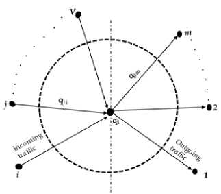
  Fig.1. Flow conservation condition

  
  

Algorithm 2 : EERPM algorithm

Start

• 1:    lifetime (  ) = 0

• 2:    compute the link quality between sensor nodes and using eqn. (3)

• 3:    if a sensor node has enough residual energy then

• 4:    compute least cost path for the current round using equations (1) and (2)

• 5:    end if

• 6:    if a node cannot get a path to the base station then

• 7:    return (Lifetime)

• 8:    stop

• 9:    else

• 10:    continue

• 11:    end if

• 12:    node forward sensed data to the base station using equation (3)

• 13:    compute the energy dissipated for individual node using equation (5)

• 14:    update residual energies of sensor nodes in their batteries

• 15:    lifetime = lifetime +1

• 16:    go to 2

End

• V. Data Extraction AND Aggregation

This section presents sensor nodes data extraction and aggregation. Subsection E presents a model for data gathering, solution to data collection problem is presented in subsection F and subsection G discusses design principle for data collection and aggregation.

• A.    Model for Data Gathering

In real WSNs applications, sensor nodes generate large amounts of data from their sensing area and store them temporarily before they are transmitted to the data collection centers for further processing. How to efficiently extract and transmit relevant data for processing becomes a new challenge in sensor networks considering resource-constraint of sensor nodes. In order to eliminate similar data and minimize transmission of large volume of data within the network, it is necessary to perform in-network aggregation as the data are moving towards the data centers. A foreign coding model in [22] is adopted to perform data aggregation during routing. In this model, a sensor node is able to aggregate the data packets transmitting from a neighbouring node with its own data. The aggregation ratio between sensor nodes and is expressed by the correlation coefficient as follows:

^ ij

R M

1--

П

where (  ) represents the encoded data packets rate at sensor node and (  |  ) represents the encoded data rate of the same data packets     at node . The correlation coefficient decreases exponentially with the distance between the sensor nodes. Based on this model, a sensor node performs two main functions on the data received from a source node . First, it compresses the data packets using its own local information. Secondly, it transmits the aggregated data to the next higher neighbouring node . Let and represent the aggregated data packets traffic at sensor nodes and respectively. The aggregated data packets traffic consist of two parts: data traffic received from the neighbouring nodes and data generated at node . Given a set of sensor nodes and denotes the base station where all the data packets are to be received. is expressed as follows:

T =§,VTj+ ” (! - n)]c,          (23)

Equation (23) shows that there exists a link from to each sensor node in the network except the (base station) and from to . Thus, the new network graph is = (  ,  ) where =   ∪ { } and =   ∪ { , } ∪

{ ,  } for all ∈  . The main aim of these expressions is to ensure data packets transmitted from a source node through a node ∈ are reliably received at the base station. It is assumed that every sensor node generates a data packet per round to be sent to the base station. A round is defined as an equal period of time allocated to the sensor nodes for data transmission and reception. Therefore, the problem of gathering maximum possible data from the resource-constrained sensor nodes can be formulated into a linear programming as follows:

Maximize      f               (24)

Subject to qM< qi max, i * A, Z(25)

X qjt=X qj jeVj

X q ER + X QijEixij < Era, VA, Z j=1

qj > 0, V(i, j)e L(28)

where equation (25) states that the amount of data sent by source node to any sensor node is less than or equal to the amount of data       transmitted from node .

Expression (26) is the normal flow conservation constraint already defined above. Equation (27) shows that the total energy consumed by a sensor node in receiving and sending data is less than or equal to the initial energy of the sensor node. A good model developed for data packets gathering must respect these constraints at each sensor node.

• B.    Solution to Data Collection Problem

The above data gathering problem is translated into a linear programming. If the link capacity between the super node and sensor nodes can be measured, then sensor nodes readings can be determined in time . If represents data flow along the link to for all ( , ) ∈  .

, denotes the data flow from super node to node and , denotes the data flow between node and through the link. ⃗⃗ = { } be the set of the incoming links of node , such that ∈ and ⃖⃗⃗⃗⃗ = {  } be the set of the outgoing links of node , such that ∈  . These statements can be translated into a linear programming as follows:

Maximize   X fA,t(29)

i e i

Subject to

X fA ,i-X j Z = 0(30)

X fj-X f = 0, Vi ± A, Z(31)

j eji on this model, a sensor node will transmit through an energy efficient path from source node to the base station so as to minimize sensor nodes’ energy consumption. The link capacity of each link is the energy required to support a successful data transmission using the link.

• C.    Design Principle for Data Collection and Aggregation

One of the ways to minimize energy consumption in WSNs is to enable individual sensor nodes to transmit through a short distance. This can be achieved by dividing the network into different groups. An approach proposed in [1] is adopted to partition the network into finite clusters . A cluster can contain one or more cluster heads and member nodes depending on the network size. In the given network, sensor nodes are given different roles to play. A member node plays a role as a forwarder node, while a CH plays a role as a data collector and a forwarder node. Initially, a desired number of cluster heads ( ) is randomly selected, since most of the sensor nodes have sufficient energy at the initial stage. A sensor node joins a CH based on the received signal strength (RSS) from each cluster head, energy consumption and bandwidth to form a cluster. Thereafter, the CH creates a time using time division multiple access (TDMA) to assign the time each member node within the cluster forwards data to it. Let be a Boolean variable. Assigning a sensor node to its corresponding CH is expressed as follows:

1if a node i is assigned to CHk bik =<

V ik such that 1 <  i <  V ,1 <  k <  K

0 otherwise

If denotes the minimum lifetime of the CH, (that is, =    {  ∀ such that 1 ≤  ≤  }) and      be the average distance between the CH and their member nodes. The average distance is expressed as follows:

d- = '/v ( rd* ) ^b *          3

The clustering problem can be translated into linear programing as follows:

ff

7+ + X % < 1, V ij e V         (32)

Cj    ij■ 'e I(ij) Cij fy< Cj, Vij e V                (33)

Equations (30) and (31) are data flow conservation constraints. Constraint (32) ensures that only a link that is interference free among other links can transmit data. Constraint (33) ensures that data flow along a link cannot be greater than the link capacity in a given round. Based

	L Maximize     k d avg	(36)
Subject to
	K
	X b lk = 1, V 1 <  i <  V k = 1	(37)

:X d _ik b _ik < T max , V 1 < i < V           (38)

k = 1

Algorithm 3 : Data transmission

Begin

1 for each frame f in round R do

• 2:    if ( i.role = collector and forwarder)

• 3:      i . forwarder ← high RSS( i.cluster );

• 4:      i.timeslot = TRUE;

• 5:   else

• 6:      i . S eepMode =TRUE;

• 7:   end if

• 8:   end for

• 9:   if ( i.role = forwarder);

• 10:   if ( i . forwarder = ) ;

• 11:     transmit to the corresponding cluster head;

• 12:     else

• 13:   collect all the data from member nodes;

• 14:   aggregate and forward to the data centre;

• 15:   Next k;

• 16:    end if

End

• Fig.2. Pseudo-code for data

Table 2. Parameters used in the simulations transmission

Parameter	Value
Number of nodes (V)	100, 200, 300, 400, 500
Network area	200 x 200 rn?
ε fs	7nJ/bit/m2
Packet size	4000 bits
ℰ	50nJ/bit
Energy for data aggregation	0.0013pJ/bit/m4
( Eda ) Energy dissipation for	5nJ/bit
processing Sensor node transmission	50nJ/bit
range	120m
Threshold distance ( dn )	75m
Cluster radius	55m
Transmit power	0.395 W
Receiving power	0.360W

• VI. Performance Evaluation

  We evaluate the performance of the proposed algorithms and models formulated with different experimental scenarios. The proposed scheme was evaluated with AEEC, MLCAL and MLCS protocols discussed in section 2. Sensor nodes in the range 100 to 500 are randomly distributed over 200 m x 200 m sensor field. The simulation runs for 65 random topologies for each network to ensure consistency of the results. The average values obtained are used for the plotting of the graphs. The linear programming (LP) models are solved using the ILOG CPLEX 12.6 studio optimization [8]. Simulation time runs for 1000 seconds for each experiment; the packet size is 4000 bits and data rate is four packets per second. Parameters and their corresponding values used in the simulation are presented in table 2. The following metrics are used to check the performance of the models formulated and compare with selected protocols.

Energy consumption: It is the energy dissipated by the sensor nodes during transmission and reception computed through simulation time.

Network lifetime: The network lifetime can be defined as the time until a certain percentage of nodes run out of battery.

Packet delivery ratio: It measures the percentage of data packets that are successfully transmitted from source nodes to the destination node.

The greater the percentage of data packets delivered, the better the performance of the protocol. The initial energy of each sensor node is varied from 1.0J to 2.0J. Each sensor node dissipates some energy from its battery whenever it receives or sends a data packet. An energy loss model with ^[j ≤ ^0 is used for short distances communication between the sensor nodes, while dij > d₀ is for long distances, ^0 is set distance threshold. A sensor node radio circuitry dissipates Eelec =50 TlJ / bit to run the receiver or transfer circuitry and ℰ amp =100 pj / bit m2 for the transmitter amplifier. We performed different sets of experiments to examine the impact of different parameters used.

• A.    Network Lifetime

Our main interest in these experiments is to determine the average lifetime of the sensor networks in each protocol. The results obtained for different network sizes with random distribution of sensor nodes for two base station locations are shown in Fig.3 and Fig. 4 respectively. The symbol “ Ｉ ” placed on top of each bar represents the standard deviation (SD). It gives the average variance between energy levels on all sensor nodes.

First, the base station is placed at the center of the network to determine the average network lifetime. The average network lifetime achieved by EERPM for a network size of 100 sensor nodes is 3.4% higher than MLCS, 10.7% higher than MLCAL and 19.5% higher than AEEC as shown in Fig. 3. Moreover, the network size increases to 500, using the same network setting, EERPM is 5.3% higher than MLCS, 23.7 % higher than MLCAL and 29.3% higher than AEEC protocols.

In another scenario, the base station is located outside the network area at the coordinate (200, 385) m for different network sizes as shown in Fig. 4. The average network lifetime achieved by EERPM is 9.3% higher than MLCS, 17.4% higher than MLCAL and 31.1% higher than AEEC for a network size of 100 sensor nodes. Similarly, the network size increases to 500, EERPM is 11.6% higher than MLCS, 18.2% higher than MLCAL and 25.0% higher than AEEC protocols. EERPM performs better in the two base station locations than MLCS, MLCAL and AEEC as shown in the figures. The reason is that sensor nodes are able to communicate with their cluster heads through short distances due to uniform distribution of cluster heads within the network. In addition, energy dissipation by each sensor node during transmission is proportional to the Qi bits sensed data and sensor nodes that are not transmitting or receiving any data and go into sleep state.

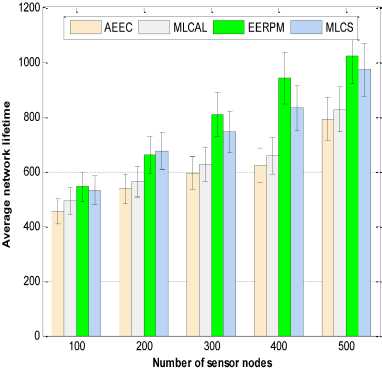
Fig.3. Average network lifetime. Base station located at the center of the network

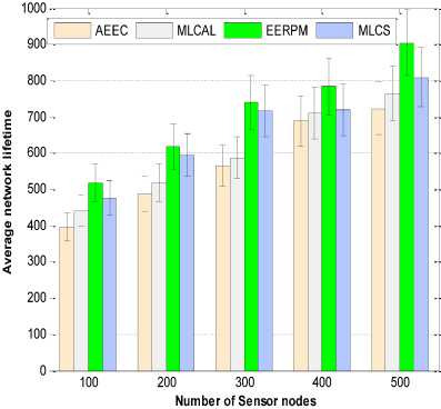
Fig.4. Average network lifetime. Base station located outside the network area

Moreover, the initial energy was varied from 1.0J to 2.0J to determine the network lifetime of the proposed method with other protocols. Simulation results for the two base station locations are presented in table 3 and table 4 respectively. In the tables, first node dies (FND) and last node dies (LND) mean the times at which the first and the last sensor nodes used up their energy and died. Half of the nodes alive (HNA) means the time at which half of the sensor nodes remain alive. The protocols dissipate their energy slowly with the number of runs. Network lifetime in each of the schemes increases as the sensor nodes’ energy increases. Thus, when the base station is placed at the center of the network, sensor nodes have longer lifetime before the FND compared to when it was placed outside the network area. In both base station locations, EERPM performs better compared to selected protocols. This is due to inclusion of some constraints such as the lower and upper bounds constraints and the residual energy constraint into the linear programming formulations.

Table 3. Sensor Networks Lifetime. Base Station is at the Centre of the Network Field

Energy (J)	Protocol	FND	HNA	LND
	EERPM	616	784	913
1.0	MLCS	607	735	882
	MLCAL	584	689	874
	AEEC	513	621	838
	EERPM	805	945	1104
1.5	MLCS	781	918	1089
	MLCAL	734	818	996
	AEEC	645	781	922
	EERPM	821	985	1182
2.0	MLCS	778	911	1160
	MLCAL	624	886	1128
	AEEC	582	795	1012

Table 4. Sensor networks lifetime. Base station is outside the network field

Energy (J)	Protocol	FND	HNA	LND
	EERPM	281	431	654
1.0	MLCS	224	398	612
	MLCAL	193	310	563
	AEEC	187	287	518
	EERPM	431	675	852
1.5	MLCS	402	624	839
	MLCAL	364	591	765
	AEEC	315	506	712
	EERPM	637	819	908
2.0	MLCS	604	772	862
	MLCAL	537	687	817
	AEEC	472	612	689

• B.    Data Packets Transmission Reliability

Data packets transmission reliability of the four protocols is investigated using a network size of 200 sensor nodes randomly distributed over the network area. Fig. 5 shows the average data packets transmission reliability taken by the sensor readings for the four schemes. EERPM presents the highest data packets reliability compared to MLCS, MLCAL and AEEC. The reason is that the proposed protocol is able to uniformly distribute the cluster heads within the network. Each sensor node belongs to a cluster with minimum energy cost. In addition, it is able to select a node that processes less data as a relay node which reduces queuing delay.

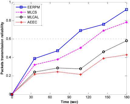
Fig.5. Data packets transmission reliability

• C.    Effect of Energy Cost

α and β are parameters used to determine the proportion of energy cost and communication cost factor respectively such that the sum of α and β is equal to 1. The values of α is varied to determine when the 1st node dies, 20% nodes die and 50% nodes die. It is observed that when the value of α is more than 0.8, it shows the moment when the first node dies. About 20% sensor nodes die when the value of α equals to 0.8 as shown in Fig. 6. In addition, 50% of sensor nodes are dead when α is in the range 0.72 to 0.76. The reason for this is that most nodes have almost exhausted their energy at these points and the remaining nodes transmit through long distance.

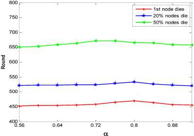
Fig.6. Effect of α value on network lifetime

Fig. 2 shows that networks total energy consumption vary with the number of sensor nodes in all the four protocols. More energy is dissipated as the size of the network increases using the same network area. The energy consumption of EERPM is less than MLCS, MLCAL and AEEC as shown in the figure. The reason is that some constraints are included into the proposed model; it only ensures a link that is interference free among the set of links can transmit data at time t . Secondly, a constraint is imposed to ensure that data flow along a link cannot be greater than the link capacity during the scheduled time t .

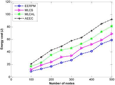
Fig.7. Total energy consumption

• D.    Average Number of Reliable Sensor Nodes

The threshold value of reliable nodes (high supportability) is assumed to be in the range 0 ≤ a2 ≤ 1. The value of ^2 is varied from 0.8 to 1.0. The average value of the reliable sensor nodes is shown in Fig. 8. The number of the reliable sensor nodes decreases as the energy of the sensor nodes decreases. Moreover, as the network size increases, the average number of redundant sensor nodes likewise increases.

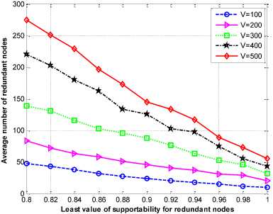
Fig. 8. Average number of reliable sensor nodes

• E.    Data Gathering Hop Selection

The effect of number of hops in a network through simulation was performed. The number of hops between the sensor nodes and the base station varied from one to three. When the number of hops increases, data gathering latency reduced as shown in Fig. 9. The reason is that when the data gathering hop is one, cluster heads only collect data from the neighbouring nodes and transmit the aggregated data to the base station. The communication distance reduces, hence it minimizes sensor nodes’ energy consumption. However, in order to have maximum network coverage, cluster heads need to collect data from member nodes that are closer to them. This reduces communication distance and data gathering latency. Thus, when the hops between the cluster heads and the base station increase, their data gathering range likewise increases. Hence, cluster heads near the base station will not only send their own data, but also transmit data received from other cluster heads. Therefore, an increase in the number of hops in a network reduces the data gathering latency as depicted in the figure.

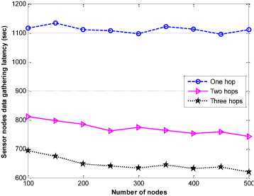
Fig.9. Data gathering latency varying number of hops

• F.    Number of Data Received at the Base Station

Fig.10 and Fig. 11 show the number of data packets received at the base stations. First, the base station is placed at the center of the network and thereafter placed outside the network field. The number of data packets received at the base stations is higher than the three schemes. This is due to some constraints such as maximum link capacity and residual energy of receiving node included into the linear programming formulations.

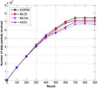
Fig.10. Total data packets received at the base station located at coordinate (100,100 ) over time

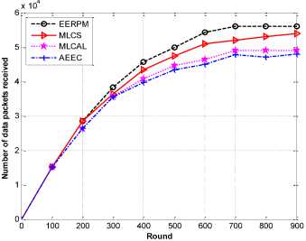
Fig.11. Total data packets received at the base station located at coordinate (200,385) over time

In Fig.12 and Fig.13, an efficient utilisation of power enables the sensor network of the proposed scheme to remain alive for a longer period compared to other protocols. Similarly, as soon as the sensor nodes begin to dissipate all their energy, the whole network ceases to function.

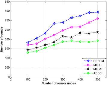
Fig.13. Number of nodes against rounds when LND

• G.    Throughput

Throughput is another metric used to measure the performance of the proposed protocol. It is the total number of data delivered over the total simulation time. The higher the value of the throughput means the better the performance of the algorithm. Fig. 14 shows the throughput of the four protocols obtained from the simulation results varying the number of sensor nodes. Thus, as the number of the sensor nodes increases, the throughput for each protocol likewise increases. The results show that EERPM has a higher throughput compared to MLCS, MLCAL and AEEC. The reason is that EERPM considered the minimum separation distance between the cluster heads and the residual energy of the relay nodes during communication.

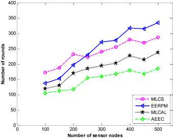
Fig.12. Number of nodes against rounds when FND

This paper presents a routing problem and formulates models for maximizing network lifetime in WSNs. Three parameters were considered in determining the energy cost for transmitting data packets between the sensor nodes: 1) the initial energy of each sensor node 2) the energy consumed for a unit data transmission flow over the communication link between two sensor nodes 3) the remaining energy of sensor nodes on the constructed path. Moreover, during data collection, interference free constraint is included into the model to ensure that only

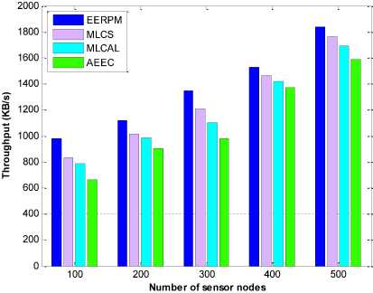
Fig.14. Number of nodes against throughput link that is free from interference can transmit data at a given time. An algorithm for optimal cluster formation and data gathering were presented. Simulation results show that the proposed scheme performed better and was able to extend network lifetime compared to selected protocols. In future, we intend to conduct research on Internet of Things and lightweight cloud computing platforms through efficient traffic engineering.

• [1]    A. P. Abidoye, "Energy optimization for wireless sensor networks using hierarchical routing techniques " PhD, Computer Science, University of the Western Cape, South Africa, 2015.

• [2]    I. F. Akyildiz and M. C. Vuran, Wireless Sensor Networks , first edition ed. New York: John Wiley & Sons, 2010.

• [3]    N. A. Alrajeh, M. Bashir, and B. Shams, "Localization techniques in wireless sensor networks", International Journal of Distributed Sensor Networks, 9, pp. 304628, 2013.

• [4]    M. S. Bandral and S. Jain, "Energy efficient protocol for wireless sensor network," In Proceedings of Recent Advances and Innovations in Engineering (ICRAIE) , Jaipur, India, 2014, pp. 1-6.

• [5]    B. Barekatain, S. Dehghani, and M. Pourzaferani, "An Energy-Aware Routing Protocol for Wireless Sensor Networks Based on New Combination of Genetic Algorithm & k-means", Procedia Computer Science, 72, pp. 552-560, 2015.

• [6]    I. Bhattcharya, P. Sarkar, and P. Basu, "RBNS Encoded Energy Efficient Routing Protocol for Wireless Sensor Network", International Journal of Information Technology and Computer Science (IJITCS), 6, pp. 65-71, 2014.

• [7]    Y. Chen, Z. Wang, T. Ren, Y. Liu, and H. Lv, "Maximizing Lifetime of Wireless Sensor Networks with Mobile Sink Nodes", Mathematical Problems in Engineering , pp. 1-13, 2014.

• [8]    I. I. CPLEX. (2013). ILOG CPLEX Optimization Studio version       12.6 .       Available:       http://www-

  01.ibm.com/support/docview.wss?uid=swg21503602

• [9]    S. Ergen and P. Varaiya, "On multi-hop routing for energy efficiency", IEEE Commun. Lett .9 , pp. 880–881, 2005.

• [10]    Heinzelman, A. Chandrakasan, and H. Balakrishnan, "An application - specific protocol architecture for wireless microsensor networks", IEEE Transactions on Wireless Communications, 1, pp. 660-670, 2002.

• [11]    S. K. A. Imon, A. Khan, M. Di Francesco, and S. K. Das, "Energy-efficient randomized switching for maximizing lifetime in tree-based wireless sensor networks", IEEE/ACM Transactions on Networking, 23, pp. 14011415, 2015.

• [12]    R. Kacimi, R. Dhaou, and A.-L. Beylot, "Load balancing techniques for lifetime maximizing in wireless sensor networks", Ad hoc networks, 11, pp. 2172-2186, 2013.

• [13]    Z. Lu, W. W. Li, and M. Pan, "Maximum lifetime scheduling for target coverage and data collection in wireless sensor networks", IEEE Transactions on Vehicular Technology, 64, pp. 714-727, 2015.

• [14]    J. K. Murthy, S. Kumar, and A. Srinivas, "Energy efficient scheduling in cross layer optimized clustered wireless sensor networks", Int’l Journal of Computer Science and Communication, 3, pp. 149-153, 2012.

• [15]    N. A. Pantazis, S. A. Nikolidakis, and D. D. Vergados, "Energy-efficient routing protocols in wireless sensor networks:  A survey", Communications Surveys &

  Tutorials, IEEE, 15, pp. 551-591, 2013.

• [16]    S. Rani, R. Talwar, J. Malhotra, S. H. Ahmed, M. Sarkar, and H. Song, "A novel scheme for an energy efficient Internet of Things based on wireless sensor networks", Sensors, 15, pp. 28603-28626, 2015.

• [17]    S. Saxena, S. Mishra, and M. Singh, "Clustering based on node density in heterogeneous under-water sensor network", International Journal of Information Technology and Computer Science (IJITCS), 5, pp. 49-55, 2013.

• [18]    N. Seddiki and A. Douli, "Maximization the lifetime of wireless sensor networks," In Proceedings of on Information & Communication Technology and Accessibility (ICTA) , Marrakech, Morocco, 2015, pp. 1-3.

• [19]    S. Singh, R. Shakya, and Y. Singh, "Localization techniques in wireless sensor networks", International Journal of Computer Science and Information Technologies, 6, pp. 844-850, 2015.

• [20]    S. Singh and A. K. Sharma, "Distributed Algorithms for Maximizing Lifetime of WSNs with Heterogeneity and Adjustable Sensing Range for Different Deployment Strategies", International Journal of Information Technology and Computer Science (IJITCS), 5, pp. 101108, 2013.

• [21]    A. K. VARGA, "LOCALIZATION TECHNIQUES IN WIRELESS SENSOR NETWORKS", University of Miskolc, Hungary Department of Automation and Communication Technology, 6, pp. 95-103, 2013.

• [22]    P. Von Rickenbach and R. Wattenhofer, "Gathering correlated data in sensor networks," In Proceedings of 2004 Joint Workshop on Foundations of Mobile Computing , 2004, pp. 60-66.

• [23]    M. Yang and A. J. Liu, "Maximum lifetime coverage algorithm based on linear programming", J. Inform. Hiding Multimedia Signal Process, 5, pp. 296-301, 2014.

• [24]    H. U. Yildiz, K. Bicakci, B. Tavli, H. Gultekin, and D. Incebacak, "Maximizing Wireless Sensor Network lifetime by communication/computation energy optimization of non-repudiation security service: Node level versus network level strategies", Ad Hoc Networks, 37, pp. 301-323, 2016.

• [25]    Y. Yun and Y. Xia, "Maximizing the lifetime of wireless sensor networks with mobile sink in delay-tolerant applications", Mobile Computing, IEEE Transactions on, 9, pp. 1308-1318, 2010.

• [26]    N. Zaman, T. J. Low, and T. Alghamdi, "Energy efficient routing protocol for wireless sensor network," In Proceedings of 16th Int'l Conf. on Advanced Communication Technology , Pyeongchang, 2014, pp. 808-814.

• [27]    L. Zhang, Q. Zhu, and J. Wang, "Adaptive Clustering for Maximizing Network Lifetime and Maintaining Coverage", Journal of Networks, 8, pp. 616-622, 2013.

• [28]    M. Zhao and Y. Yang, "Optimization-based distributed algorithms for mobile data gathering in wireless sensor networks", Mobile Computing, IEEE Transactions on, 11, pp. 1464-1477, 2012.