Energy Resource Management of Assembly Line Balancing Problem using Modified Current Search Method

Conventionally, effective energy resource management consists of energy management program, organization structure, energy policy, planning, auditing and reporting [1]. Moreover, classical method for energy resource management uses the various principles such as energy management system (EMS), excess energy management (EEM), energy driven force (EDF), energy knowledge management (EKM), energy innovation creation (EIC), energy system control (ESC)

and energy organization culture (EOC) [2]. The conventional orientation focuses on operations and activities done by human. However, due to human uncertainty in operation, those approaches seem inefficient and non-sustainable. Generally, energy resource management conducted recommendations of consultants usually based on their experience and feeling. The motivation of this research is initiated from needs to find the general algorithm to solve the energy resource management in industries efficiently.

Regarding to optimization context, many of challenging applications in science, engineering and technology can be formulated and performed as optimization problems [3,4]. Energy management can be considered as a class of non-polynomial time hard (NP-hard) combinatorial optimization problem. Such the problem usually possesses nonlinear and unsymmetrical terms as well as multiple local solutions. These cause the problem complex and difficult to solve by an exact method within a reasonable amount of time. Moreover, inefficient algorithms are easily trapped due to its local solutions. To solve the problem, metaheuristic optimization methods are alternatives [4].

Over five decades, many efficient metaheuristics such as genetic algorithm (GA), tabu search (TS), particle swarm optimization (PSO), harmony search (HS) and current search (CS) have been developed for combinatorial, continuous and multiobjective optimization problems [5]. These algorithms can be classified into two groups: population-based and singlesolution based algorithms. Two important properties of any metaheuristics are exploration and exploitation [68]. Exploration property simply means the generation of diverse solutions to explore the search space on the global scale, while exploitation focuses on the search in a local region by exploiting information that a currently good solution is found in a local region. It was found by literatures that the population-based has strong exploration property, while the single-solution based has strong exploitation property. Metaheuristics has been widely applied to various real-world engineering problems [5,7]. One of the latest metahueristic search algorithms is the current search (CS) [9]. By literatures, the CS has been successfully applied to control engineering [10] and signal processing [11]. The CS performed satisfactory results. However, the CS may be trapped by local optima. Therefore, the CS algorithms need to be modified to improve its effectiveness.

This paper proposes the adaptive current search (ACS), which is the modified version of the CS method as a new tool for solving the resource management optimization problems. It consists of five sections. The ACS algorithms are elaborately explained in section II. The performance evaluation of the ACS over five benchmark unconstrained and three constrained optimization problems compared with GA, TS and CS is provided in section III. The application of the ACS to energy resource management of the assembly line balancing (ALB) problems is illustrated in section IV, while conclusions are given in section V.

• II.    Adaptive Current Search Algorithms

The current search (CS) has been developed based on the principle of current divider in electric circuit theory [9,10,11]. The behavior of electric current is like a tide that always flow to lower places. The less the resistance of branch, the more the current flows. The CS algorithm is described by the flow diagram represented in Figure 1. The advantages are that the CS can find any local solution in each search direction efficiently. Moreover, it can provide unlimited search directions defined by users. However, the CS algorithm is based on an electric current behavior considered as the natural movement. The disadvantages of the CS are that its search process may be trapped or locked by any local solution. In addition, the search time consumed by the CS is depended on the numbers of search directions.

The modified version of the CS algorithm is called the adaptive current search (ACS) metahueristics. The memory list (ML) and the adaptive radius (AR) mechanism are proposed for inserting into the CS algorithms. The ML is used to escape from local entrapment caused by any local solution, while the AR is conducted to speed up the search process. The proposed ML consists of three levels: low, medium and high. The low-level ML is used to store the ranked initial solutions at the beginning of search process, the medium-level ML is conducted to store the solution found along each search direction, and the high-level ML is used to store all local solutions found at the end of each search direction.

Once the search process is started, the set of initial solutions is generated randomly. They will be ranked by the objective function of the problem of interest from most to least significant. The ranked initial solutions will be stored in the low-level ML. This scheme helps the ACS algorithms to be stronger in exploration strategy.

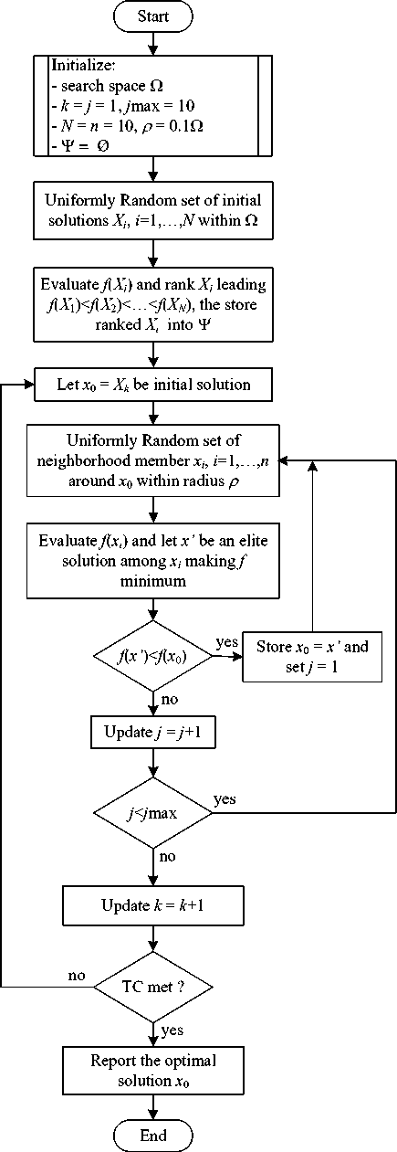
Fig. 1: Flow Diagram Of CS Algorithm [9]

The ranked initial solution with most significant will be selected as the current solution for the first search direction. The neighborhood members will be generated randomly around the current solution within the certain radius. All neighborhood members will be evaluated by

the objective function of the problem. The best neighborhood giving the minimum objective function value is used to compare with the current solution. If the best neighborhood is better than the current solution, the current solution will be replaced by the best neighborhood, while the previous current solution will be keep into the medium-level ML. Once the search process moves close to the local solution (which can be observed by the objective function value), the AR mechanism is activated to speed up the process. The search radius is thus reduced according to the objective function value found so far. The less the objective function value found, the smaller the search radius is adapted. This implies that the refined solutions will be considered. Then, the local solution of this search direction will be found within faster time and will be keep into the high-level ML. This scheme helps the ACS algorithms to be stronger in exploitation strategy.

After the local solution of the first search direction is found, the search process look backward to the low-level ML. The second most initial solution ranked in the low-level ML will be selected as the current solution for the second search direction so far. This scheme will be repeated until the global solution will be found or the termination criteria are met.

With ML and AR mechanism, a sequence of solutions obtained by the ACS rapidly converges to the global minimum. The developed ACS algorithms can be described step-by-step as follows:

Step 1 Initialize the search space Ω , iteration counter k = j = 1, maximum allowance of solution cycling j max , number of initial solutions N , number of neighborhood members n , search radius R , and low-level ML Ψ = ∅ , medium-level ML Γ = ∅ , and high-level ML Ξ = ∅ .

Step 2 Uniformly random initial solution X i , i = 1,…, N within Ω .

Step 3 Evaluate the objective function f ( X i ) for ∀ X . Rank X i that gives f(X 1 ) <  — <  f(X N ), then store ranked X i into the low-level ML Ψ .

Step 4 Let x 0 = x k as selected initial solution.

Step 5 Uniformly random neighborhood x i , i = 1,…, n around x 0 within radius R .

Step 6 Evaluate the objective function f ( x i ) for ∀ x . A solution giving the minimum objective function is set as x *.

Step 7 If f ( x *)< f ( x ₀), keep x ₀ into medium-level ML Γ _k and set x ₀ = x *, set j = 1 and return to Step 5. Otherwise keep x * into medium-level ML Γ _k and update j = j +1.

Step 8 If the search process moves close to the local solution, activate the AR mechanism by adjusting R = ρR , 0< ρ <1.

Step 9 If j < j max , return to Step 5. Otherwise keep x 0 into high-level ML Ξ and update k = k +1.

Step 10 Terminate the search process when the termination criteria (TC) are satisfied. The optimum solution found is x 0 . Otherwise return to Step 4.

ACS algorithms mentioned above can be represented by the pseudocode as shown in Figure 2, and some movements of the ACS search process can be depicted in Figure 3.

Pseudo-code of ACS procedure

Initialize the search space = Ω , the memory lists (ML) Ψ = Γ = Ξ = ∅ , the iteration counter i = j = k = l = 1, the maximum search iteration in each direction I max , the maximum allowance of solution cycling j_max , the number of initial solutions (feasible directions of currents in network) N , number of neighborhood members n , the maximum objective function value ε for AR, and the search radius R .

while ( i <  N ) do // generate search directions Generate initial solutions X _i randomly within Ω; Evaluate f ( X i ) via the objective function; Rank X _i giving f ( X _i ) from min to max values ( X 1 gives the min, while X N gives the max objective function values); Store ranked X _i into Ψ;

end_while while (k ≤ N) or the TC are not satisfied do

Set x 0 = X k ;

while ( i ≤ I max ) do

Generate neighborhood x k,l ( l = 1,2,…, n ) randomly around x ₀ within R ;

for l ← 1 to n do

Evaluate f ( x k,l ) via the objective function; Set x * as a solution giving the minimum objective value;

end_for if f(x*) < f(x0) do

Keep x 0 into Γ k ;

Set x 0 = x *;

Set j = 1;

else do

Keep x * into Γ k ;

Update j = j+ 1;

end_if if f(x0) < ε do // activate the AR Adapt R = ρR, ρ ∈ [0, 1];

end_if if j == jmax do // activate other directions Keep x0 into Ξ;

Update k = k+ 1;

Go out-loop while ;

end_if

Update i = i+ 1;

end_while

Keep x 0 into Ξ;

Update k = k+ 1;

end_while end_procedure

Fig. 2: Pseudocode Of ACS Algorithm

Y (Low-level ML) = I QIО | О | СУ|

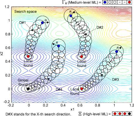
Fig. 3: Some Movements Of ACS Algorithm

• III.    Performance Evaluation

• 3.1    Unconstrainted Optimization

This section presents the performance evaluation of the ACS against unconstraint and constraint benchmark optimization problems compared with GA, TS and CS. The efficiency of those algorithms can be measured by the success rate of finding the global optima. In this paper, algorithms of GA and TS are omitted. Readers may refer to [12,13] for GA and [14,15] for TS, respectively. Those algorithms were coded by MATLAB running on Intel Core2 Duo 2.0 GHz 3 Gbytes DDR-RAM computer, while GA is used from the MATLAB-GA Toolbox [13]. Each algorithm performs search on each test function for 100 trials beginning with different initial solutions while search parameters are kept the same. Search parameter settings for the GA follow MATLAB-GA Toolbox [13] and for the TS follow [15].

For unconstraint optimization test, GA, TS, CS and ACS are tested against five well-known unconstrained optimization problems [16] including Bohachevsky function (BF), the fifth function of De Jong (DJF), Griewank function (GF), Michaelwicz function (MF) and Shekel’s fox-holes function (SF). These problems are summarized in Table 1, in which J min is the minimum values of objective functions required to terminate the search. The search parameters of the CS and the ACS for this test are set as summarized in Table 2, where n = number of neighborhood members, R = search radius, N = search (current) paths and I max = maximum search iterations.

Table 1: Summary Of Unconstrained Optimization Problems

BF:      f ( x , y ) = x ² + 2 y ² - 0 . 3 cos( 3 nx ) - 0 . 4 cos( 4 ny ) + 0 . 7

global minimum located at x = 0, y = 0 with f ( x , y ) = 0, search space: x,y g [-2, 2] and J min < 1 x 10^-6

where a ^ =

- 32 - 16    0   16   32 - 32 - 0 16 32 ^

- 32 - 32 - 32 - 32 - 32 -16 - 32 32 32 J global minimum located at x = -32, y = -32 with f(x,y) = 0.9980, search space: x,y g [-40, 40] and Jmin < 0.9990

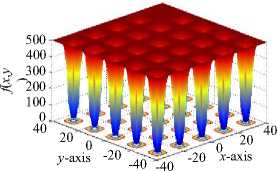
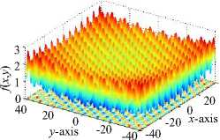
GF:    f (x, У) = 1 + {(1 / 4000)( x2 + У 2)} - {cos(x )cos(y / Л)} global minimum located at x = 0, y = 0 with f(x,y) = 0, search space: xy g [-40, 40] and Jmin < 1 x 10-6

MF:     f ( x , y ) = - sin( x )sin ²⁰ ( x ² / n ) - sin( y )sin ²⁰ ( 2 y ² / n )

global minimum located at x =2.20319, y = 1.57049 with fx,y) = -1.8013, search space: xy g [0, 4] and Jmin < -1.80129

-1

• -24  _{3   2}

y -axis   ¹   _{0  0}

1 x -axis

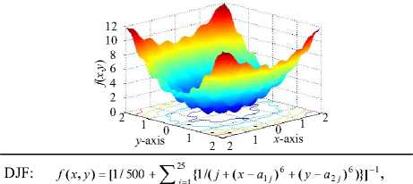
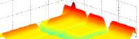
SF:      f ( x , y ) = - ^ 3°, [ 1 /{ C j + ( x - ° 1 j ) 2 + ( у - ° 2 j ) 2 }],

where

a ij =

9 . 6810 9 . 4000 8 . 0250 - 9 . 4960 4 . 13 80

0 . 6670 2 . 0410 9 . 1520 - 4 . 8300 2 . 5620

C j = ( 0 . 8060 0 . 5170 0 . 1000 0 . 9080 - 0 . 6080 0 . 3260 ) global minimum located at x =8.0241, y = 9.1465 with f ( x , y ) =

-12.1190, search space: xy g [0, 10] and J min <-12.1189

-2

-4

-6

-8

-10

• -12₁₀

5 y -axis

Table 2: CS and ACS Parameter Setting

CS Parameter Settings
Test functions	n	R	N	I max
BF	50	0.1	50	1,000
DJF	50	5.0	100	1,000
GF	100	0.5	100	1,000
MF	50	2.0	50	1,000
SF	100	1.5	50	1,000

ACS Parameter Settings
Test functions	n	R	N	I max	R – adjustment
					S t a g e I	Stage II
BF	50	0.1	50	1,000	J < 1 × 10-2 → R = 0.01	J < 1 × 10-4 → R = 0.001
DJF	50	5.0	100	1,000	J < 1 × 102 → R = 1.00	J < 10 → R = 0.50
GF	100	0.5	100	1,000	J < 1 × 10-2 → R = 0.01	J < 1 × 10-4 → R = 0.001
MF	50	2.0	50	1,000	J < 1 → R = 0.01	J < 0 → R = 0.001
SF	100	1.5	50	1,000	J < -2 → R = 1.00	J < -5 → R = 0.50

Table 3: Results of Unconstrained Optimization Problems

Test functions	GA	TS	CS	ACS
BF	480,100 ± 34,612(86%)	465,100 ± 19,745(96%)	241,310 ± 9,867(100%)	200,250 ± 7,572(100%)
DJF	385,400 ± 26,748(77%)	352,520 ± 21,632(94%)	124,212 ± 8,410(98%)	112,028 ± 7,046(100%)
GF	902,150 ± 67,223(82%)	780,464 ± 41,947(92%)	514,575 ± 31,108(96%)	501,020 ± 21,663(100%)
MF	200,375 ± 22,591(88%)	145,680 ± 10,866(95%)	67,260 ± 3,103(99%)	49,640 ± 2,458(100%)
SF	685,450 ± 45,411(90%)	545,120 ± 33,012(97%)	325,850 ± 14,102(100%)	302,210 ± 9,815(100%)

Results obtained are summarized in Table 3, where the global optima are reached. The numbers are in the format: average number of evaluations (success rate). For example, 200,250±7,572(100%) means that the average number (mean) of function evaluations is 200,250 with a standard deviation of 7,572. The success rate of finding the global optima for this algorithm is 100%. Referring to Table 3, it can be observed that the ACS is much more efficient in finding the global optima with higher success rates. For all test functions, the proposed ACS outperforms GA, TS and CS.

• 3.2    Constrainted Optimization

For constraint optimization test, GA, TS, CS and ACS are tested against three constrained optimization problems consisting of Fcon01, Fcon02 and Fcon03, detailed as follows.

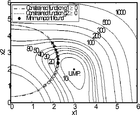
The function Fcon01 [17] is stated in equation (1). This function is a minimization problem with two design variables and two inequality constraints. The unconstrained objective function f(x) has a minimum solution at (3, 2) with a corresponding function value equal to zero. The constrained minimum solution is located at x* = (2.246826, 2.381865) with an objective function value equal to f*(x) = 13.59085.

min f ( x ) = ( x ₁ + x ₂ - 11 )   + ( x ₁ + x ₂ - 7 )

x subject to, g1(x) =4.84-(x1 - 0.05)2 -(x2 -2.5)2 ≥0,     (1)

g ₂ ( x ) = x ₁ + ( x ₂ - 2 . 5 )   - 4 . 84 ≥ 0 ,

0 ≤ x ₁ ≤ 6 ,   0 ≤ x ₂ ≤ 6

For this function, parameter settings for the GA follow MATLAB-GA Toolbox [13] and for the TS follow [15]. The common search parameters of the CS are: n = 1,000, R = 0.1, N = 500 and Imax = 1,000. Jmin ≤ 13.60 is the minimum values of objective functions required to terminate the search. For the ACS, R- adjustment is set as J< 25.00 ^ R = 0.01 and J< 15.00 ^ R = 0.001. Results are summarized in Table 4 and Figure 4.

Direction-1 Direction-2 Direction-3

U.M.P. = Unconstrained MinimumPoint

Fig. 4: Movements Of ACS Algorithm Over Fcon01

From Figure 4, it was found that the ACS spent only three search directions to reach the global optimum. Table 4 shows the best solutions found by the GA, TS, CS and ACS as well as their corresponding objective function values. It was noted that the ACS result is very close to the optimal solution and outperforms other three results not only in the aspect of the objective function values but also in that of constraint accuracy.

The function Fcon02 [18] with two design variables and two constraints is stated in equation (2). The minimum solution is located at x * = (0.82288, 0.91144) with an objective function value equal to f *( x ) = 1.3935.

Once GA follows MATLAB-GA Toolbox [13] and TS follows [15]. The common parameters of the CS are: n = 1,000, R = 0.1, N = 500 and I max = 1,000. J mn <  1.3936 is the minimum values of objective functions required to terminate the search. For the ACS, R -adjustment is set as J < 5.00 ^ R = 0.01 and J < 2.00 ^ R = 0.001. Results are summarized in Table 5. It was found that the ACS outperforms other three results in both the objective function values and the constraint accuracy.

Table 4: Results Of Fcon01 Constrained Optimization Problem

Algorithms	Optimal solutions x *		Constraints		Objective function f *( x )
	x 1	x 2	g 1	g 2
GA	2.246840	2.382136	0.00002	0.22218	13.590845
TS	2.2468258	2.381863	0.00002	0.22218	13.590841
CS	2.2468262121	2.3818704379	2.21003 X 10-15	0.2221826212	13.5908416934
ACS	2.246828512562	2.381813302772	1.8332002 X 10-18	0.2221828329242	13.590841501204030

Table 5: Results of Fcon02 Constrained Optimization Problem

Algorithms Optimal solutions x* Constraints Objective function f*(x) x 1 x 2 g 1 g2 GA 0.8350 0.9125 1.0 X10-2 -7.0 X10-2 1.3772 TS 0.8343 0.9121 5.0 X10-3 5.4 X10-3 1.3370 CS 0.82283310 0.91144165 1.0 X10-6 4.9 X10-6 1.3935867 ACS 0.82283256086 0.91142060358 -8.6463030 X10-6 4.9127562X10-5 1.39356948924 min f (x) = (xi - 2)2 + (x2 -1)2 x

minf (x) = (xj -10)2 + 5(x2 -12)2 + x34

x

+ 3(x4 -1 1)2 +10x56 + 7x62 + x 4

- 4 x 6 x 7 -10x 6 - 8 x 7

subject to,

g 1 (x) = 127-2x 1 - 3x2 -xз - 4x4 -5x5 — 0,

g2(x) = 282-7x 1 -3x2 -10x3 -x4 + x5 — 0,

g3 (x) = 196- 23x 1 - x2 - 6x2 + 8x7 — 0,

g 4 (x) = -4 x 1 - x 2 + 3 x1 x 2 - 2 x3 - 5 x6 + 11x 7 — 0,

• -10

  
  

Like Fcon01 and Fcon02, parameter settings for the GA follow MATLAB-GA Toolbox [13] and for the TS follow [15]. The common search parameters of the CS are: n = 2,000, R = 0.1, N = 1,000 and Imax = 1,000. Jmin < 680.63 is the minimum values of objective functions required to terminate the search. For the ACS, R-adjustment is set as J < 1,000 ^ R = 0.01 and J < 750 ^ R = 0.001. Results are summarized in Table 6. It was found also that the ACS outperforms other three algorithms and provides superior results.

Table 6: Results Of Fcon03 Constrained Optimization Problem

Optimal solutions x * and Objective function f *( x )	GS	TS	CS	ACS
x 1	2.32345617	2.33047	2.33087488	2.324971068354062
x 2	1.951242	1.95137	1.95136990	1.950016515825672
x 3	-0.448467	-0.47772	-0.47459349	-0.491430343898877
x 4	4.3619199	4.36574	4.36555341	4.370929879461707
x 5	-0.630075	-0.62448	-0.62452549	-0.623883321164803
x 6	1.03866	1.03794	1.03793634	1.040859835982587
x 7	1.605384	1.59414	1.59406525	1.593387864833378
f *( x )	680.6413574	680.6380577	680.6350771	680.6304164174447

m

• IV.    ACS Application to ALB Problems

The application of the ACS to energy resource management of the assembly line balancing (ALB) problems is proposed. The ALB problem is considered as one of the classical industrial engineering problems [19]. An assembly line is a sequence of workstations connected together by a material handling system. It is used to assemble components or tasks into a final product. The fundamental of the line balancing problems is to assign the tasks to an ordered sequence of workstations that minimize the amount of the idle time of the line, whereas satisfying two particular constraints. The first constraint is that the total processing time assigned to each workstation should be less than or equal to the cycle time. The second is that the task assignments should follow the sequential processing order of the tasks or the precedence constraints.

The ALB can be considered as the class of combinatorial optimization problems known as NP-hard [20,21]. In this work, the single-model assembly line balancing problem is considered. Balancing of the lines can be measured by the idle time (Tid), the workload variance (wv) and the line efficiency (E) [22]. Therefore, the goals of balancing assembly lines are to minimize the idle time and the workload variance. Analytical formulations for the ALB problems are stated in equations (4) - (7), where m is the number of workstations, W is the total processing time, c is the cycle time and Ti is the processing time of the ith workstation.

m = W / c(4)

m

Td =Z (c - Ti)(5)

i = 1

Wv = - XT — W / m )]2

i = 1

E = УТЛ m x c)

i = 1

The ALB problem can be formulated as the multiobjective constrained optimization problem. The multiobjective function ( J ) consisting of the workload variance ( w v ) and the idle time ( T id ) is performed as stated in equation (8), where γ 1 and γ 2 are weighted factors ( γ 1 + γ 2 = 1.0). J in equation (8) will be minimized by the ACS metaheuristics as expressed in equation (9).

J = Y1 x wv + Y2 x Tid minimize J subjectto  T < c, precedentconstrains

By this approach, the workload variance will be minimized in sense of the resource management optimization. This implies that, if all machines (once one machine, one workstation is assumed) of the assembly line are equally operated, resource management is optimal. This means that the assembly line of interest is balanced and all machines possess the same workload. Again by this approach, the idle time will be minimized in sense of the energy management optimization. This implies that, if all machines of the assembly line are operated with full-time production (without or with the least idle time), energy management is optimal. In contrast, running some machines without production is the energy loss of the line. In this application, the proposed ACS associated with the heuristic sequencing (HS) technique is conducted to solve the ALB problems. The proposed ACS is used to address the number of tasks assigned for each workstation, while the HS technique is conducted to assign the sequence of tasks for each workstation according to precedence constraints as represented by Figure 5.

The HS is based on the heuristic logics of practicing engineers to arrange the sequence of tasks assigned for each workstation. In practice, assigning task will be considered from its processing time, number of succeeding tasks and number of precedent tasks. The proposed PH algorithm is thus described as follows.

Step 1 Let number of tasks be n .

Step 2 Initialize sequence of tasks Δ = ∅ and i = 1.

Step 3 If a current task, δ i , possesses properties:

• (3.1)    no precedent tasks,

• (3.2)    maximum succeeding tasks, and

• (3.3)    maximum processing time, put δ i into Δ respectively, delete δ i , n = n – 1, then go to Step 4, otherwise, update i = i + 1, then go back to Step 3.

Step 4 If n = 0, terminate the sequencing process. The sequence of tasks stored in Δ is successfully arranged, otherwise set i = 1, go back to Step (3).

workstation set for the corresponding search spaces. Once the search process stopped, results obtained are summarized in Table 9.

Table 7: Details of Benchmark ALB Problems

Entry	Name	n	W (min.)	c (min.)	m
1	Buxey	29	324	50	7
2	Sawyer	30	324	40	9
3	Warnecke	58	1,548	160	10
4	Tonge	70	3,510	325	11

Table 8: Lists of Search Spaces

Entry	Search spaces
1	S 1 ∈ [2, 7]; S 2 ∈ [3, 8]; S 3 ∈ [2, 6]; S 4 ∈ [3, 7]; S 5 ∈ [2, 7]; S 6 ∈ [2, 5]; S 7 ∈ [2, 5]
2	S 1 ∈ [2, 5]; S 2 ∈ [2, 6]; S 3 ∈ [3, 6]; S 4 ∈ [3, 6]; S 5 ∈ [2, 5]; S 6 ∈ [1, 4]; S 7 ∈ [1, 5]; S 8 ∈ [1, 4]; S 9 ∈ [2, 5]
3	S 1 ∈ [3, 6]; S 2 ∈ [3, 6]; S 3 ∈ [4, 8]; S 4 ∈ [6, 9]; S 5 ∈ [5, 9]; S 6 ∈ [3, 6]; S 7 ∈ [4, 7]; S 8 ∈ [5, 8]; S 9 ∈ [5, 8]; S 10 ∈ [4, 8]
4	S 1 ∈ [6, 9]; S 2 ∈ [5, 8]; S 3 ∈ [2, 6]; S 4 ∈ [3, 6]; S 5 ∈ [5, 7]; S 6 ∈ [3, 6]; S 7 ∈ [5, 10]; S 8 ∈ [6, 12]; S 9 ∈ [6, 12]; S 10 ∈ [5, 8]; S 11 ∈ [5, 8];

Note: S i stands for the i ^th workstation.

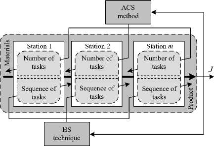
Fig. 5: ACS-Based ALB Problem Solving

The proposed approach is tested against four benchmark single-model ALB problems collected by Scholl [23] as summarized in Table 7. In this work, the number of workstations, m , can be calculate by equation (4). For all tests, the parameter settings for the GA follow MATLAB-GA Toolbox [13] and for the TS follow [15]. The common search parameters of the CS are: n = 1,000, R = 0.2 and I max = 1,000. N = 500 is required to terminate the search. For the ACS, R -adjustment is set as I max = 500 → R = 0.1 and I max = 750 → R = 0.01. The CS and ACS algorithms were coded by MATLAB running on Intel Core2 Duo 2.0 GHz 3 Gbytes DDR-RAM computer. The γ 1 = γ 2 = 0.5 are set to compromise the w_v and T_id in equation (8). Table 8 provides the boundaries of number of tasks for each

Table 9: Results of ALB Problems

Entry 1:		Buxey
Apps.	w v	T id (min.)	E (%)
GA	11.06	26.00	94.46
TS	8.77	26.00	95.02
CS	2.64	26.00	95.38
ACS	1.35	26.00	96.42
Entry 2: Sawyer
Apps.	w v	T id (min.)	E (%)
GA	6.00	36.00	90.00
TS	5.84	36.00	91.85
CS	3.22	36.00	95.47
ACS	1.56	36.00	97.30
Entry 3: Warnecke
Apps.	w v	T id (min.)	E (%)
GA	18.56	52.00	95.66
TS	10.11	52.00	95.91
CS	8.86	52.00	96.04
ACS	6.56	52.00	97.35
Entry 4: Tonge
Apps.	w v	T id (min.)	E (%)
GA	11.54	65.00	98.18
TS	8.74	65.00	98.85
CS	3.98	65.00	99.01
ACS	1.17	65.00	99.40

Note: Apps. stands for approaches.

Table 10: Results of Tonge-ALB Problems by ACS

Work-	Tasks assigned	Station
Station	for each	Time	(min.)
( m )	workstation	(min.)
1	1,2,3,5,9,15,24	317	8
2	4,6,7,10,41,68	319	6
3	11,16,18	318	7
4	8,12,14,30,69	318	7
5	13,17,19,20,22,57	319	6
6	21,23,25,27	320	5
7	26,29,31,32,33,34,58,59	320	5
8	28,35,36,37,38,44,45,48,51,70	319	6
9	39,40,56,61,62,63,64	320	5
10	42,43,46,47,49,52,67	321	4
11	50,53,54,55,60,65,66	319	6

The total idle time ( T id ) = 65.00 min., The workload variance ( w v ) = 1.17, The line efficiency ( E ) = 99.40%.

Referring to Table 9, it was found that the proposed ACS associated with the HS technique is capable of producing solutions superior to other techniques for all ALB problems. The workload variance, w v , can be successfully minimized in sense of the resource management optimization, while the idle time, T_id , can be satisfactory minimized in sense of the energy management optimization. For example, Table 10 contains the results of the Tonge-ALB problem obtained by the ACS with HS association in details.

• V.    Conclusions

The application of the adaptive current search (ACS) to energy resource management optimization has been proposed in this paper. The ACS is the modified version of the current search (CS) developed from the behavior of an electric current flowing through electric networks. With the memory list (ML) and the adaptive radius (AR) mechanism, the ACS effectiveness can be improved to escaping from any local entrapment and to speed up the search process. For its performance evaluation against five benchmark unconstrained and three constrained optimization problems compared with genetic algorithm (GA), tabu search (TS) and CS, it was found that the ACS outperforms other algorithms and provides superior results which are very close to the optimal solutions for all testes functions. The proposed ACS has been applied to energy resource management of the assembly line balancing (ALB) problems associated with the heuristic sequencing (HS) technique. By this approach, the ACS is applied to address the number of tasks for each station, while the HS technique is used to assign the sequence of tasks according to precedence constraints. The workload variance (wv) and the idle time (Tid) are formed as the multipleobjective function for this application. As results from four benchmark ALB problems compared with the GA, TS and CS, it was found that the ACS associated with the HS technique is capable of producing solutions superior to other techniques for all ALB problems. The workload variance can be successfully minimized in sense of the resource management optimization, while the idle time can be satisfactory minimized in sense of the energy management optimization. This can be concluded that the proposed ACS is an alternative powerful algorithm to solve the ALB problems in sense of energy resource management and other optimization problems.