Enhanced deep feed forward neural network model for the customer attrition analysis in banking sector

Published Online July 2019 in MECS

The paper is structured as follows. Section 2 explores the various literature reviews on the related work. Section 3 explains the various research objectives of the proposed work. Section 4 and 5 illustrates the methodology and results of the proposed work. Section 6 explores the conclusion and future work.

• II.    Related Works

This segment investigates on the related work which has been as of now done in the territory of customer attrition analysis forecast utilizing different classes of machine learning model in the different area, for example, telecom, retail industry, and Banking domains.

In [4] the customer attrition model is implemented using the decision tree for the Banking domain. One of the fundamental points in utilizing the decision tree is it is easy to build and interpret this model. The CRISP technique is utilized in building the prescient model. The models are validated using the Receiver operating characteristic curve. The feature determinations are done by using the technique of forwarding selection and backward elimination. An exactness of 85% is acquired with this model when the model is presented to the set number of data. In any case, the restriction of the work is, as the colossal volume of the data is more, the execution of the model debases because of the overfitting of the tree.

The Artificial neural network based model is implemented in [5] to predict the customer attrition in the Banking segment. The Bank dataset was taken from the UCI website. The proposed research work is implemented in rapid miner simulator. The Neural Network model is built using 3 hidden layers with nine input neuron, and 2 output neuron to yield the outcome. The general exactness of 78.18% is gotten with this model.

In [6] hybrid combination of Support vector machine with random forest are used to predict the customer attrition. The support vector machine is an administered learning technique where hyperplanes are utilized to separate between various classes. The point is to make the biggest edge with hyperplane to separate between the classes in high dimensional space. Bigger the edge, bring down the mistake on prediction result. In the random forest, ensembling systems are pursued where as opposed to building the single model, numerous models are assembled, the exactness of these models are combined to get a more steady forecast. The proposed work is done by using the MATLAB tool where dataset had 3333 rows and the aggregate of 21 properties. The ensemble model obtained a satisfactory result compared with the individual model.

The customer attrition model is implemented utilizing the blend of the diverse machine learning algorithms in [7].The investigation is carried out using the collaboration of JRip algorithm and K means clustering. The work is conducted in the WEKA simulation tool. The dataset was collected from the banks of Nigeria. The dataset had about one lakh client record with 11 distinct properties. The dataset was preprocessed using the weka software. Dataset was partitioned into the train and test sets and models were trained using the training examples. To start with, the informational collection is passed to the k implies bunches, after creating the distinctive arrangement of groups, the information are broke down utilizing JRIP classifier. The model gave valuable learning to the bank which is helpful information with respect to value-based conduct of customers which, helped the banks to examine the churners.

In [8] Neural Network model is implemented using Alyuda Neuro Intelligence simulator to predict the customer attrition. The idea behind the model was that the model forecasted the attrition result based on the on the quantity of the product selected by the customer. In the event that the customer utilizes under 3 products of the Bank, such customers are anticipated as churners. The Neural simulator is built having 3 hidden layers with eight neurons, four neurons, and two neurons in each of the hidden layers and it is presumed that individuals who are youthful and having under three products of the bank are probably going to be churners.

In [9] the churn predictions are performed using deep learning models for the telecom space. Three profound neural systems convolution neural network, feed-forward neural system, Large Feedforward neural are framed. The two diverse telecom informational datasets are passed to these profound learning models. An exactness of 71.66% is acquired with Large feed forward neural system and convolution neural system. Test results demonstrate that the profound learning models perform similarly as SVM.

The idea of customer attrition analysis even connected to the domain of telecommunication. In [10] the customer churn analysis is made using the diverse set of machine learning algorithms Naïve Bayes, Logistic Regression, Decision Tree, and Artificial Neural Network. The information is gathered from the five media transmission organization. The rapid miner simulator is used to build the model. The information is pre-processed, information types are changed over into the numeric qualities for the predictive analysis. Before passing the information to the machine learning model, the FP Growth algorithms are used to get the relationship between the qualities. A similar investigation is made by running the informational collection utilizing five diverse models. The C5.0 furnished the ideal exactness of 85 %.

In [11] customer churn is predicted using the extreme gradient boosting algorithm (XGBoost). The transactional and subscription data considered as input to the model. The informational collection is separated into Training and Test set. The model is validated using a crossvalidation technique. The dataset is also validated using log loss model. The data set had 208 features. The features which expand the precision of the model are held and undesirable are disposed of. The model implemented using XGBoost library utilizing the Python. Overall exactness/accuracy of 79.7% is acquired with the test information.

In [12] Customer attrition related to the retail sector are analyzed using deep learning based model. The profound learning models are shaped utilizing a limited Restricted Boltzmann machine(RBM) and convolution neural network(CNN). The POS value-based data sets are used to conduct the experiment. The dataset has undergone the procedure of ETL. Anomalies are expelled from the dataset before isolating the dataset into preparing and testing. After the evacuation of exceptions, the informational collection is partitioned arbitrarily in 75:25 proportion where 75 show training set and 25 demonstrate the test set. The informational dataset is passed as input to the Restricted Boltzmann machine and the convolution neural network. The point is to check whether accuracy is reliant on chronicled information. Total 30 iterations carried through the training set and sigmoid is used as activation function, an accuracy of 74% is achieved. Using RBM an accuracy of 83% is accomplished.

In [13] churn analysis for the telecom information is made using the PSO based simulated annealing. The prescient exactness of the proposed methodology is compared with the decision tree, Naive Bayes, support vector machine, K-nearest neighbor, random forest. Trial results uncover that the execution of the proposed metaheuristics is progressively productive contrasted with the other machine learning model.

In [14] the customer attritions in the telecom sector is made using the firefly algorithm. Each firefly is contrasted with each other firefly with dependent on the power of the light. Firefly calculation due to their metaheuristic nature can distinguish ideal arrangement viable. The investigation is led on the orange informational dataset of French telecom organization. The power of the firefly is processed utilizing reenacted toughening. The real disadvantage of these algorithms is the colossal computational prerequisite, where Firefly should be contrasted and each other firefly on every emphasis.

In [15] dynamic behavioral model is proposed to predict the churn rate in the financial sector. The dynamic model is implemented based on behavioral traits and spatio temporal patterns. The credit card transactional data from the major financial institution are used to conduct the experiment. In the proposed paper new entropy of choice based feature selection method is implemented to select the useful features from the given data set. The experimental results show that the proposed dynamic behavioral model performed significantly better than the traditional way of predicting the churn rate in the financial sector.

In [16] a big analytics based framework is implemented to predict the churn rate among retiree segment in the Canadian banking industry. The proposed model is built in the Hadoop platform using the decision tree algorithm. The main objective of the paper was to construct the predictive churn data model by utilizing the big data. Hence 3 million customer record is collected from the various sources like online web pages. The SAS business intelligence software is used to analyze the input data set. The experimental results showed that the proposed model performed better result in terms of accuracy compared to the existing approaches.

• III.    Objective of the Work

According to the writing review completed in the segment 2 it has been seen that the current machine learning based model which are connected to foresee the churn prediction are computationally costly in nature since it needs to emphasize over the extensive volume of preparing dataset until the point that the model merges and another issue with these model is it performs inadequately with high – dimensional client information and furthermore these model are one-sided with the classes that have a substantial number of case. Thus they will, in general, foresee the dominant part class information, not with minority class information. Subsequently to defeat these issues the proposed work is conveyed with the following objectives.

• 1)    To use optimized one hot encoding and Tukey outliers algorithms to perform the feature selection and the preprocessing.

• 2)    To Perform the greedy forward feature selection on this encoded information to select the best feature to enhance the accuracy of the prediction result

• 3)    To tune the hyperparameter of the proposed model automatically during the model preparing process.

• 4)    To achieve ideal accuracy with machine learning

model utilizing powerful enhancement technique like Adam optimizer.

• IV.    Proposed Methodology

In the proposed work Enhanced Deep Feed Forward Neural Network(EDFFNN) based model are built to forecast the customer attrition in the Banking sector. The customer churn data set is taken from the UCI machine learning archive. The dataset has total 10,000 customer churn data with 14 dimensions of features. The Exit variable of the dataset indicates the customer churn where twofold factor 0 shows that the customer remain and 1 demonstrate that the customer leaves the current Banking Organization.

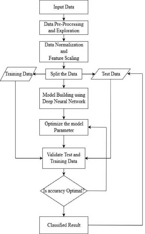
Fig.1. Proposed architecture Diagram

The architectural design of the proposed methodology is as appeared in figure 1 underneath. As a component of the initial step, the customer churn information is passed as input to the proposed Model. The pre-processing stage includes outlier detection using the Tukey outlier detection algorithm[17]. The Tukey Outlier works based on the Interquartile range (IQR) to distinguish the outliers in the given dataset. This technique does not rely upon any standard deviation or the factual mean and henceforth the extraordinary scope of qualities in the given informational collection can be dealt with utilizing this calculation. The autonomous variable of the dataset like the client id, surname, and column number isn't considered as there is no effect on the needy variable. Since the model needs the contributions to numerical information, the dataset is encoded where the straight out information is changed over into numerical information utilizing one hot encoding and mark encoding procedure. It is one of the methods utilized to get higher performance[18].

The advantage of data exploration is the relation between the data is visually represented in terms of the graphs or the diagram. Since this present reality dataset has highlighted with high variability in their sizes, ranges, and the units, standardization must be performed to scale the element which is unessential or deluding. The Euclidean distance between the data features are measured and then it will be normalized. It is a vital step which can be connected to standardization of the information and to scale up the highlights for the quicker computation[19]. As the standardization and feature scaling on the given dataset completed, model is built using deep feed-forward neural network algorithm by bringing in the keras library with the input layer, output layer and hidden layers in it. The Deep Feed Forward Neural Network model is implemented with 5 hidden layers in it. Each of the hidden layers contains six internal nodes in it which are made dependent on the number of features in the data set.

The Weights are instantiated automatically utilizing the kernel initializer. The activation function is used in the Neural Network to achieve non-linear behavior otherwise it acts like a simple linear regression model or the linear model. The role and softmax are used as activation function for the hidden layers, which is optimal[20] where the problem of vanishing gradient are avoided. The sigmoid activation function performs best in the output layer, hence the same activation function is applied to the output layer. The sigmoid activation function ranges between [0,1].To test the precision of the model, a whole dataset is portioned into 2 sections. In the greater part, 80% of the information is kept for training model and 20% of the data set is passed as the input test set for the model. The primary reason behind this is to avoid data overfitting.

The Neural Network model is initialized with weights using an adaptive weight strategy where weights are automatically assigned to the data features of the neural network node and the learning rates are controlled using Adam optimizer algorithms. The expansion of the traditional stochastic gradient descent is Adam optimizer which is used in deep learning based model. The Adam optimization algorithm requires less memory space and at the same time, it is computationally efficient. The performance of Adam optimizer is better than RMSProp[21]. The Adam optimizer is well suited for the problems wherever there is sparse or noisy data and also it requires the lesser hyperparameter. One more advantage of using Adam optimizer is the learning rate which is automatically tuned based on the network weights.

In the proposed EDFFNN model the log loss based binary_crossentropy is made use to quantify the performance of the model. The binary_crossentropy yields the result in binary 0 and 1. The loss will increases if the prediction result deviates from the actual results. In order to avoid the overfitting and the underfitting problems of the machine learning model, the validation data sets are used. The proposed neural network model is continuously trained using the training example with a total of 100 epochs. The epoch indicates the forward and backward pass through the training examples. The Batch size indicates the total number of training instances involved in the given epoch. As increasing the size of the batch the more memory spaces occupation increases. The anticipated prediction result is changed in to genuine if the expectation of the prediction outcome >0.5 else it is considered as False. On the off chance that the ideal precision is not gotten, the hyperparameter of the profound learning models like the input layers, number of units of the node in the layers, kernel_intializers are refreshed until the point that the ideal exactness is acquired.

The steps profound in building the neural network model is as follows.

Stage 1: The input layer of the neural network node are fed with features of the data sets as indicated in equation 1 below.

N[0]= F                   (1)

where N indicates the input node of the neural network and F indicate the features passed through the node.

Stage 2: The feature weights are assigned to each of the neural nodes which is dot product between weights and the features indicated in equation 2 below.

N[i]= Weight[i]*F               (2)

Equation 2 illustrates that input features are multiplied with weights. The value of the weight depends on the feature importance.

Stage 3: The edge is created between the input layer and the hidden layer by using equation 3 below.

input_hidden_layer= Weight[i]* F         (3)

Stage 4: The hidden layers are activated by using ReLu and softmax activation functions. The layers are activated from left to the right for the forward propagation as shown in equation 4 and 5 below.

activation_hidden_layers=ReLu(hidden_layer)(4)

activation_hidden_layers=Softmax(hidden_layer)(5)

Stage 5: The input to the output layer is the dot product between the hidden layer activation and weighted feature as indicated in equation 6 below.

Input_output_layer=(activation_hidden_layers *Weight[i])(6)

Step 6 : The error propagated by subtracting the actual result with the obtained result

Err=Actualoutput-Predicted output

Step 7 : The feature Weights are automatically updated using optimal adaptive Adam optimization strategy. The weights are tuned using learning rate as a measure.

Step 8 : Repeat the step number from 1 to 5 and an adaptive weighting strategy is continuously applied using Adam optimizer algorithms

Step 9 : The entire training set is gone through the process of the deep feed-forward neural network and the until the point when it results in maximal accuracy with prediction result.

• V.    Result and Discussion

To assess the prediction accuracy of the proposed enhance deep feed-forward neural network model, the whole data set is portioned in training and test set with the proportion of 80: 20. The model is prepared/trained using 80% of the preparation/training precedents. The test sets are passed to the proposed model in order to test or to validate the models. The results obtained through prediction are compared with actual figures/statistics. The validation of the model is done using the parameters ROC curve, F1 score, recall, precision and confusion matrix to avoid the data overfitting and underfitting and biased result.

The F1 score is viewed as critical to identify the Biased prediction result with the given Model. It works based on the false positive and false positive statistics of the prediction model. The equation to ascertain the F1 score is given underneath.

F1Score=2* (Precision*Recall)/(Precision+Recall) (8)

The confusion matrix is one more measure to evaluate the correctness of the machine learning model. The outcome with the confusion matrix is a false negative, false positive, true positive and true negative. The predictive accuracy of the classification model can also be validated using ROC(Receiver Operating Characteristic) curve. It indicates the relations between recall and precision value. It represents the false positive in terms of X-axis and true positives in Y-axis. The ROC curves are quantified by total AUC rate(Area under curve) which ranges between 0 and 1.

The section below explores on results obtained through the proposed enhanced deep feed-forward neural network model when the Bank churn data set are passed as input to this model.

The proposed Enhanced deep feed-forward neural network model built with five layers in it. Every layer of the neural network is implemented with six nodes. The number of neural nodes is dependent on the dimension and features of the data set. The Bank churn data set is passed as input to the model. The entire data set is divided into 10 different batches. Total of 100 epochs done through the batches. The model epoch and model accuracy diagrams got through the proposed model is as appeared in figure 2 and 3 underneath.

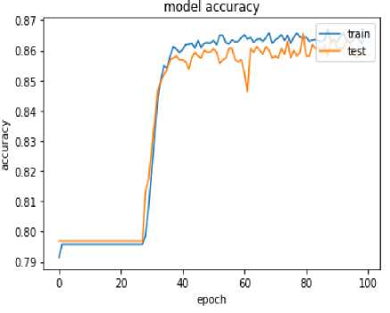
Fig.2. Model Epoch Vs Accuracy with EDFFNN

Figure 2 indicates that the accuracy of 86.23% is obtained through the training set and 85.29% accuracy achieved with test data.

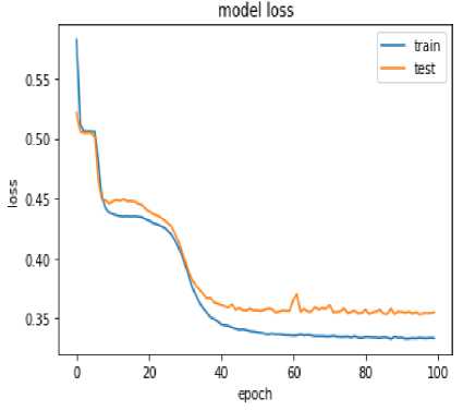
Fig.3. Model Epoch Vs loss with EDFFNN

Figure 3 shows that as epochs carried through the training examples and there is a decrement in the model loss hence the increase in accuracy. The model is trained by tracing 100 epochs through the training examples. The model epoch and loss graph indicate that at the 100th epoch the loss with respect to model is below 5% in training data and it is 10% with test data.

The confusion matrix results of the proposed EDFFNN model is as shown in table 1 below. There are 82 False negative and 196 False positive, 209 True positive and

1513 True negative prediction are obtained with the proposed model.

Table 1. Confusion matrix with the proposed EDFFNN.

True Label	Negative	True Negative	1531	False Positive	82
	Positive	False Negative	196	True Positive	209
		Negative		Positive
		Predicted Label

The ROC curve for the proposed EDFFNN is shown in Figure 4. The area under the curve rate of 0.865 is achieved with the proposed model.

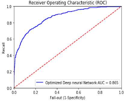
Fig.4. ROC curve of EDFFNN

The Recall, F1 score and Precision values of the proposed model are indicated in table 2. The value 0 in the table below indicate the customer who likely to continue with the same Banking organization and value 1 indicate the customer who is churners may likely to exit the current Banking organization.

Table 2. Precision, Recall, F1 score and Support with proposed EDFFNN

	precision	recall	F1 score	support
0	0.88	0.96	0.93	1592
1	0.72	0.53	0.63	408
micro avg	0.87	0.87	0.87	2000
macro avg	0.81	0.74	0.77	2000
weighted avg	0.86	0.88	0.85	2000

The comparative analysis is done with the result obtained through the proposed deep feed-forward neural network with the other machine learning algorithms such as Decision Tree, Logistic Regression, Gaussian Naïve Bayes and Artificial Neural Network. The section below explores the result obtained with this model using the same Bank churn Data set.

• A.    Decision Tree

The Decision Tree is a supervised machine learning algorithm which predicts the class label of given data by applying decision rule. The Decision tree follows the tree-like structure where each leaf node represents the class label and internal node represent the attributes. The Bank churn data set is passed as input to the Decision Tree Model. The confusion matrix obtained using the decision tree model with the Bank churn Dataset is shown in table 3 below.

Table 3. Confusion Matrix with the Decision Tree

True Label	Negative	True Negative	1533	False Positive	61
	Positive	False Negative	332	True Positive	76
		Negative		Positive
		Predicted Label

The ROC curve obtained with the decision tree is shown in figure 5 below. The AUC rate 0.675 and accuracy of 78.4% are achieved with this algorithm.

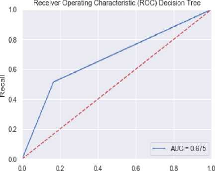
Fall-out (1-Specificity)

Fig.5. ROC curve of Decision Tree

The Recall, F1 score and Precision values obtained with the decision tree model is indicated in table 4.

Table 4. Precision, Recall, F1 score and Support with the Decision Tree Model

	precision	recall	F1 score	support
0	0.88	0.81	0.85	1582
1	0.44	0.50	0.44	418
micro avg	0.75	0.75	0.75	2000
macro avg	0.63	0.64	0.63	2000
weighted avg	0.72	0.75	0.75	2000

• B.    Logistic regression

The Logistic regression algorithm is a statistical machine learning model which uses a logistic function to perform the binary classification. Using the algorithm an accuracy of 80.15% obtained with the churn data set. Table 5 below illustrates the confusion matrix obtained with Logistic Regression.

Table 5. Confusion Matrix with the Logistic Regression

True Label	Negative	True Negative	1563	False Positive	36
	Positive	False Negative	365	True Positive	44
		Negative		Positive
		Predicted Label

The ROC curve obtained with logistic regression model shown in figure 6 indicates an AUC rate of 0.541.

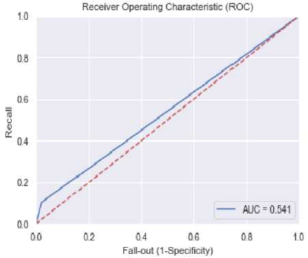
Fig.6. ROC curve of a logistic regression model

The Recall, F1 score and Precision values obtained with logistic regression model are indicated in table 6 below.

Table 6. Precision, Recall, F1 score and Support with the Logistic Regression Model.

	precision	recall	F1 score	support
0	0.82	0.96	0.87	1590
1	0.56	0.11	0.15	410
micro avg	0.81	0.81	0.81	2000
macro avg	0.67	0.53	0.52	2000
weighted avg	0.74	0.79	0.72	2000

• C.    Gaussian Naïve Bayes

The Gaussian Naïve Bayes algorithm is an extension to the traditional naïve Bayes classifier which supports the continuous and real value features where the model conforms to the Gaussian Distribution. Since the raw data used in the proposed work are real-valued input, the Gaussian Naïve Bayes(GNB) can be applied to build the model. The Gaussian Naïve Bayes takes the real-valued points as input and it calculates the mean and standard deviations of input(x) for each of the class to obtain or to summarize its distributions. Using this algorithm prediction accuracy of 81.35% is obtained which is better compared to all the baseline models. The confusion matrix obtained with Gaussian Naïve Bayes is as shown in table 7 below. With the Gaussian naïve Bayes 1536 true negative and 76 true positive instances and also 331 false negative 60 false positive misclassified instances are obtained.

accuracy and model loss graphs for the neural network model is as shown in figure 8 and 9. Figure 8 illustrates that with the training set accuracy of 83.59 % and with test data, an accuracy of 82.9% is obtained with the neural network model.

Table 7. Confusion Matrix with the Gaussian Naïve Bayes

True Labe l	Negative	True Negative	1536	False Positive	60
	Positive	False Negative	331	True Positive	76
		Negative		Positive
		Predicted Label

The ROC curve of the model shown in figure 7 below. The ROC curve is plotted using True positive rate and the False positive rate. The True positive rate is plotted along the Y axis and False positive rate is plotted along X-axis. The degree of separability is measured based on the value of AUC. The AUC rate of 0.574 is obtained with Naïve bayes model.

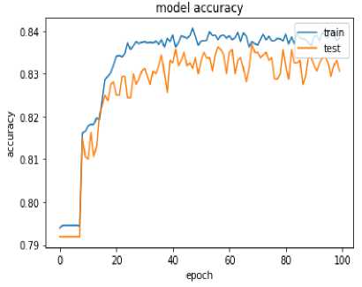
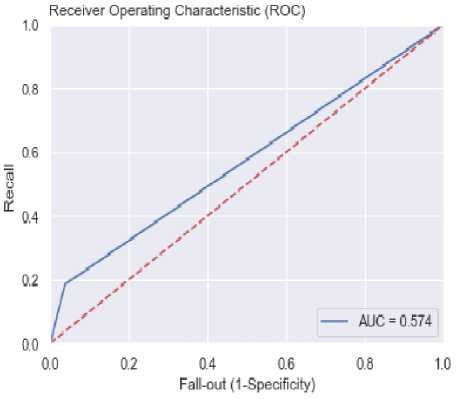
Fig.7. ROC curve of Gaussian Naïve Bayes model

The Precision, Recall, and F1 score obtained with the Gaussian Naïve Bayes model is shown table 8 below.

Table 8. Precision, Recall, F1 score and Support with the Gaussian Naïve Bayes.

	precision	recall	F1 score	support
0	0.81	0.95	0.83	1590
1	0.52	0.13	0.21	410
micro avg	0.80	0.80	0.80	2000
macro avg	0.68	0.56	0.52	2000
weighted avg	0.76	0.82	0.72	2000

• D.    Artificial Neural Network

The Artificial Neural Network(ANN) is a class of machine learning algorithm which mimic the behavior of the human brain. The experiment is extended using the basic artificial neural network model with the input layer and the single hidden layers in it. The relu is used as an activation function in the input layer and sigmoid as activation function in the output layer. An accuracy of 83.59% is obtained with the tra ining set. t he model

Fig.8. Model Accuracy Vs Epoch with Artificial Neural Network

The Model Loss with epoch graph shown in figure 9 depicts that there is the decrement in the model loss as epochs carried through the training examples hence it resulted in the increment in the accuracy with each of the epochs.

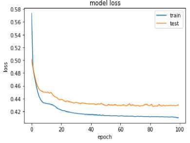
Fig.9. Model loss Vs Epoch with Neural Network

The confusion matrix obtained through ANN is shown in table 9 below. Total 1575 true negative and 124 True positive predictions and also 263 False negatives, 34 False positive predictions are obtained with the confusion matrix for the neural network.

Table 9. Confusion Matrix with the Artificial Neural Network.

True Label	Negative	True Negative	1575	False Positive	34
	Positive	False Negative	263	True Positive	124
		Negative		Positive
		Predicted Label

Total of 100 epochs is carried through the ANN model. As each epoch made through the training examples the accuracy tends to increase and there is a decrement in the model loss. The ROC graph obtained through the ANN

Model is shown in figure 10. The AUC rate of 0.739 is obtained with neural network model shown in figure 10 below. The AUC rate is larger compared to the Decision tree, Logistic Regression, Gaussian Naïve Bayes and lesser compared to the proposed EDFFNN model.

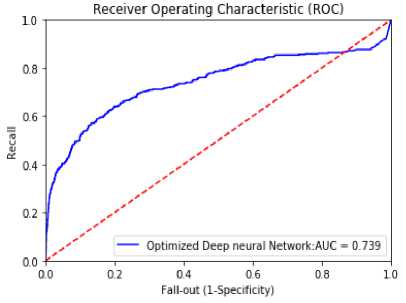
Fig.10. ROC curve of Artificial Neural Network

The Precision, Recall and F1 score obtained with the Neural Network model is shown below.

Table 10. Precision, Recall, F1 score and Support with the Artificial Neural Network.

	precision	recall	F1 score	support
0	0.85	0.96	0.90	1610
1	0.75	0.31	0.45	390
micro avg	0.84	0.84	0.84	2000
macro avg	0.81	0.64	0.67	2000
weighted avg	0.83	0.84	0.81	2000

The table 11 below shows the comparison between the proposed enhanced deep feed-forward neural network model with other class of machine learning model in terms of precision, recall and F1 score. The result depicts that the proposed model performs best compare to all other machine learning model.

Table 11. Precision, Recall and F1 score comparison of Machine Learning Model.

Machine Learning Model	Precision		Recall		F1 Score
	0	1	0	1	0	1
Enhanced Deep Feed Forward Neural Network	0.88	0.72	0.96	0.53	0.93	0.63
Artificial Neural Network	0.85	0.75	0.96	0.31	0.90	0.45
Logistic Regression	0.82	0.56	0.96	0.11	0.87	0.15
Gaussian Naïve Bayes	0.81	0.52	0.95	0.13	0.83	0.21
Decision Tree	0.88	0.44	0.81	0.50	0.85	0.44

Table 12 below illustrated the accuracy and the AUC rate comparison between the proposed Enhanced Deep Feed Forward Neural Network and other class of machine learning model.

Table 12. Accuracy Comparison between different Machine Learning Model

Machine Learning Model	Accuracy: Test Data	AUC Rate
Enhanced Deep Feed Forward Neural Network(EDFFNN)	85.9%	0.86
Artificial Neural Network(ANN)	82.6%	0.73
Logistic Regression(LR)	80.15%	0.54
Gaussian Naïve Bayes(NB)	80.3%	0.57
Decision Tree(DT)	78.4%	0.67

The bar plots in figure 11 illustrate that proposed Enhanced Deep Feed Forward Neural Network performs best in AUC rate and also in terms of the predictive accuracy compare to other predictive machine learning model.

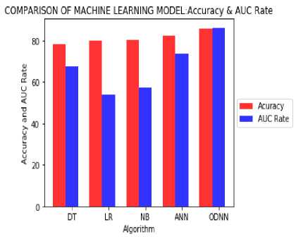
Fig.11. AUC rate and Accuracy comparison between the proposed model with different predictive learning Algorithms

• VI. Conclusion

In this paper, the Enhanced Deep Feed Forward Neural Network based model is proposed to predict the attrition rate in the Banking Sector. The enhancement to the traditional Deep Neural Network model has been done using the optimized data preprocessing, data exploration, feature scaling, and Adam optimizer algorithms. The proposed model is validated using the various measures such as a confusion matrix, ROC curve, Precision, Recall, F1 score, and log loss model. The comparative analysis between the proposed model with other class of machine learning algorithms. The result shows that the proposed model is outperformed in terms of accuracy and AUC rate compare to all the existing approaches. So it can be concluded that the proposed Enhanced Deep Feed Forward Neural Network Model is the best predictive model to analyze the customer attrition rate in the Banking Sector. As future work, the ensembling based Neural Network model can be implemented to further improve the predictive accuracy.