Enhanced Deep Learning Prediction Framework using Improved Golden Eagle and Fire Hawk Optimization

Medical insurance cost prediction plays a crucial role in enhancing transparency in the healthcare industry, where a wealth of patient data, disease profiles, and diagnoses are generated regularly. Health insurance policies serve as a safeguard, mitigating the financial impact of various health-related risks. The costs associated with healthcare and insurance are influenced by a multitude of factors. Accurate predictions of individual healthcare expenses are of utmost importance to a wide range of stakeholders and health authorities [1]. Precise cost estimates empower health insurers and healthcare organizations to strategically plan for the future and allocate their limited care management resources effectively [2]. Furthermore, providing patients with insights into their anticipated future expenses aids them in making informed decisions about insurance plans, deductibles, and premiums, contributing to the development of user-friendly insurance policies. Machine learning (ML) has the potential to enhance policy efficiency in the insurance sector and excel in predicting high-cost, high-need patient expenditures in healthcare. However, the complexity of healthcare costs, often arising from rare diseases, presents a challenge in estimating expenses. Various machine learning methods are employed in the prediction process, but their accuracy remains a limitation. These methods, while proficient at uncovering hidden patterns, are hampered by extended training periods that hinder real-time application. To address this,

This work is open access and licensed under the Creative Commons CC BY 4.0 License.

there is a growing effort to develop a deep learning-based health insurance prediction model, offering improved efficiency for policy-making in the insurance sector.

In a study detailed in [2], regression approaches are used to forecast medical insurance costs based on patient demographic and biological characteristics. Four regression techniques, namely Adaboost, elastic net, gradient boosting, and lasso, are employed for predictive modeling. This innovative system aims to facilitate the creation of user-friendly medical insurance plans that enhance revenue and user benefits. In [3], a novel approach to estimating insurance medical costs is introduced, relying on the piecewise-linear method and utilizing the SGTM neural structure. This approach enables the efficient processing of large volumes of data, ensuring high precision and rapid training. The healthcare sector grapples with the challenge of accurately predicting medical insurance costs using traditional ML techniques. As a solution, deep learning methods, particularly deep neural networks, are leveraged in [4] to address the limitations of ML regression models by effectively handling large datasets and providing accurate forecasts for insurance costs. Deep learning algorithms, increasingly employed in medical applications, demonstrate notable effectiveness in forecasting high-cost, high-need patient expenditures within the healthcare sector.

In the contemporary landscape, bio-inspired optimization algorithms are gaining more attention due to their superior performance. These algorithms, such as ant colony optimization (ACO), genetic algorithm (GA), wolf optimization algorithm (WOA), and particle swarm optimization (PSO), are explored for feature selection. Hence, this paper introduces the modified Fire Hawk Optimization (FHO) algorithm for feature selection, demonstrating its ability to select essential attributes and achieve optimal fitness values. FHO proves versatile, extending its application to solving engineering-related challenges, emphasizing its capacity to balance exploration and exploitation while searching for the ideal feature subset [5]. Enhancements in convolutional neural networks (CNNs) are achieved through techniques like dynamic chunk-based max pooling (DCMP) for pooling and improved golden eagle optimization (IGEO) for weight enhancement, resulting in an improved CNN used for predicting extracted features from medical datasets.

Although the proposed model incorporates multiple algorithmic components, their integration follows a unified design objective that addresses three major limitations commonly observed in healthcare cost prediction models. First, healthcare datasets often contain redundant or weakly informative attributes that may reduce prediction accuracy and increase computational complexity. The BFHO based feature selection stage is therefore introduced to identify the most relevant subset of features before model training. Second, conventional CNN architectures rely on static pooling operations that may not effectively capture varying feature distributions present in heterogeneous medical datasets. The DCMP strategy is incorporated to adaptively preserve informative feature patterns while reducing dimensionality. Third, the performance of deep learning models strongly depends on optimal parameter tuning, and gradient based optimization may converge to local minima when training on relatively small structured datasets such as insurance records. To overcome this limitation, the IGEO algorithm is employed to enhance CNN weight optimization through its global search capability. By assigning each optimization mechanism to a specific stage of the learning pipeline including feature relevance discovery, feature representation enhancement, and parameter optimization, the proposed framework forms a coordinated architecture rather than a simple aggregation of techniques. This stage wise hybridization ensures that the feature space is first refined, then effectively represented, and finally optimally learned, which collectively improves prediction accuracy and computational efficiency.

The major contribution of this paper is explained below:

• •    Initially, in data pre-processing, the Z-score technique is utilized to transform the original data into a useful format. And the data splitting methodology segments the datasets into calibration and prediction sets.

• •    Then, the modified FHO (BFHO) feature selection algorithm helps to improve the efficiency of the predictive model by selecting the most relevant features from the pre-processed datasets, contributing to better model performance and potentially reducing computational costs.

• •    Finally, a novel improved CNN is employed for predicting the health insurance from the feature selected datasets. The improved CNN is the hybridization of DCMP technique for enhancing the CNN network, and the IGEO algorithm’s search ability is employed to enhance the weights of CNN.

2.    Related Works 3.    Proposed Feature Selection Method

The remainder of this article is detailed in the below section. The literature review is explained in section 2. The proposed methodology is detailed in section 3 that includes pre-processing, feature selection and prediction. Then section 4 explains the experimental result and the last section 5 briefly explains the conclusion of this article.

Xue et al. [6] proposed a particle swarm optimization (PSO) in terms of multi-objective for feature selection. The existing feature selection method faces a main challenge, which is a single objective issue. To overcome this issue, the multi-objective PSO is introduced and it is able to reach better performance for feature selection issues. One of the current metaheuristic optimization algorithms is whale optimization algorithm (WOA), which imitates whale hunting mechanism. The WOA faces many issues through several other optimization methods. Tubishat et al. [7] introduced the improved WOA method. This paper presents two improvements for WOA: one is elite opposition-based learning (EOBL) that is used in the WOAs’ initial phase. Then another one is differential evolution method that is involved at the end of WOA. The humming distance based binary particle swarm optimization is proposed by Banka [8]. This method is used to improve the particles’ velocity in binary PSO framework to choose the main feature subset. However, the increasing over fitting and computational time are the main drawbacks of the optimization algorithm. To avoid these issues, this article presented the improved FHO algorithm for feature selection. This FS algorithm only selects the optimal features so it reduces the computational time and avoids over fitting.

The computational intelligence technique is proposed in Hassan et al. [9] for forecasting the cost of medical insurance. This approach can resolve the wide range application issues in the healthcare sector. However, the computational intelligence contains the groups of techniques so it mostly causes the over fitting issue. In order to estimate a person's future medical expenses, Sushmita et al. [10] proposed a model based on the medical and past expense history of a person. Moreover, to forecast the costs, they employed linear regression analysis and random forest techniques. This proposed model was used to estimate quarterly expected costs for the next 3, 6, 9, and 12 months. However, this proposed method does not reduce the prediction error. The application of the scientific state-of-art is used to detect and prevent fraud. So, Akbar et al. [11] proposed the extreme gradient boosting (XGB) algorithm for forecasting the healthcare insurance fraud. Further this proposed algorithm is utilized to develop the accuracy of a decision tree classifier. Compared to the random forest technique, the XGB approach gives more prediction accuracy. However, it takes more time for the error prediction. In Morid et al. [12], a convolutional neural network (CNN) architecture is employed to automatically discover hidden temporal patterns from multivariate time series data in patient insurance claims in order to create an efficient and scalable individual-level patient cost prediction technique. Krishnamurthy et al. [13] created and assessed a number of AI-based models in their work, taking into account minimal characteristics including sex, age, comorbidities, and medication. After six or twelve months, these models forecast a patient's chance of acquiring chronic renal disease. Additionally, the tree-based LightGBM model was utilized to determine which properties are most significant for prediction. The existing prediction model contains various problems.

Hollmann et al. [14] proposed the Tabular Prior-data Fitted Network, a foundation model designed specifically for tabular data prediction tasks. The model demonstrates superior prediction accuracy on small datasets and significantly reduces training time compared with traditional machine learning methods. Muhammed Shibil et al. [15] investigated deep learning based tabular models including TabTransformer and TabNet for electric vehicle energy consumption prediction. Their experimental results show that the TabTransformer model achieves higher prediction accuracy compared with conventional machine learning techniques. Hole et al. [16] proposed a hybrid prediction framework combining TabNet and Transformer XGBoost for traffic flow prediction in smart city environments. The study demonstrated that TabNet provides more stable performance and improved prediction accuracy compared with the hybrid model. Liu et al. [17] introduced an interpretable TabTransformer based architecture for electricity load forecasting using heterogeneous tabular data. Their proposed model improves prediction accuracy and model robustness while effectively handling categorical features and missing values.

Although these existing studies provide effective solutions for tabular data prediction tasks, many approaches still face challenges related to feature redundancy, computational complexity, and model parameter optimization. Therefore, this study proposes an improved CNN based deep learning framework integrated with the IGEO optimization algorithm to enhance prediction accuracy while reducing computational complexity in medical insurance cost prediction.

Fig. 1 illustrates the flowchart of the proposed prediction model. The initial step of the proposed approach involves data preprocessing, where the Z-score normalization technique is applied to transform the raw data into a more suitable format. Subsequently, the data is split into two distinct sets: the training set and the testing set. This division is crucial as it enables the model to learn from one set and validate its predictions on another, ensuring the robustness of the predictive model. Next, the feature selection is a critical component in enhancing the efficiency of the predictive model. In this research, the novel feature selection algorithm known as modified Fire Hawk Optimization (BFHO) is introduced. BFHO plays a significant role in reducing the number of features used for prediction, which not only enhances the model's performance but also potentially reduces computational costs. The proposed deep learning model leverages Convolutional Neural Networks (CNNs) for the prediction task. To further improve the CNN's performance, two techniques are introduced. The first is the Dynamic Chunk-Based Max Pooling (DCMP) method, which is employed to enhance the pooling layer within the CNN network. This technique assists in reducing the dimensionality of the feature vectors, ultimately decreasing computational requirements. The second technique is the Improved Golden Eagle Optimization (IGEO) algorithm, which focuses on enhancing the weights of the CNN. IGEO is a swarm-based metaheuristic optimization algorithm designed to optimize the CNN's weights. This optimization step aims to improve the model's overall predictive accuracy.

Dataset

Data Pre-processing using z-score

Feature selection using modified FHO

Prediction using improved CNN

Predicted value

Fig. 1. Flowchart for proposed approach

• 3.1.    Data Pre-processing

The initial step involves converting the raw data into a more convenient format through a preprocessing technique based on z-score normalization within the proposed model. Z-score normalization typically relies on the standard deviation of the original data to standardize the ultimate score. This Z-score normalization does not remove noisy data but instead rescales the feature values so that they have a mean of zero and a standard deviation of one. This standardization helps ensure that features with different numerical ranges contribute equally during model training and prevents attributes with larger magnitudes from dominating the learning process. Therefore, in the proposed framework Z-score normalization is used to standardize the dataset and improve numerical stability during model training rather than to eliminate noise from the data. This normalization method is particularly effective when one has prior knowledge of the matcher's mean score and the potential score range. Equation 1 represents the normalized score as follows:

New value = (^-^)                                         (1)

<7

• A.    K-Fold Cross-Validation

A widely recognized method for cross-validation is the K-fold approach. In this method, the entire dataset is randomly and uniformly divided into k separate folds or subsets. During each iteration, one fold is selected as the test data, while the remaining folds are combined to form the training data. This process is repeated until each fold has been utilized as the test data, effectively running the testing procedure k times. The effectiveness of the proposed technique was assessed by employing the K-fold cross-validation approach in the conducted studies, with the value of k set to 10.

• B.    Data Splitting

• 3.2.    Feature Selection by Boolean Fire Hawk Optimizer (BFHO)

Data splitting is a method employed to divide datasets into two distinct sets: the training (or calibration) set and the testing (or prediction) set. Typically, this division takes place after the spectra of the samples have been adjusted to mitigate distortion and unwanted variations during the preprocessing stage. The training dataset encompasses all the data used to train the model, while the testing dataset contains the data used to evaluate the trained and validated approach. It serves as a measure of the overall model's accuracy and its potential for making incorrect predictions.

The FS method, termed BFHO, commences by utilizing the split datasets. It employs the training set to identify pertinent features, initiating this procedure by establishing a population comprising N solutions and computing the fitness value for each. Subsequently, it selects the most favorable solutions and integrates them with FHO operators to refresh the population X. The subsequent phase entails choosing the relevant features from the testing set, guided by the binary representation of the best solution. The dataset used in this study contains a relatively small number of input variables. The feature selection stage is therefore incorporated not only to reduce dimensionality but also to identify the most influential attributes contributing to insurance cost prediction. Even in datasets with limited features, certain variables may contribute less to the predictive task or introduce redundancy that can affect model generalization. The BFHO algorithm evaluates different feature combinations and selects the subset that produces the lowest prediction error when used by the CNN model. Hence, the feature selection component in the proposed framework focuses on improving feature relevance and prediction robustness rather than only reducing computational complexity.

• A.    Generating Population

A population denoted as X, comprising N solutions, is created. Each solution, denoted as X_i where i ranges from 1 to n, is characterized by d dimensions. The value of each X_i is determined using the following equation to establish the initial population.

X-лч

— l j + Г ^ X (Uj —

i = 1,2, ...,n

]' = 1,2, ...,d

• B.    Updating Solutions

In the search space, the minimum and maximum values are represented by l j and U j . Then the BFHO algorithm is used to update the initial population X. The following Equation is used to transform each X_i into a Boolean form.

f 1 if X_y>0.5 ВХц — )

10 otherwise

Subsequently, the features within the training set that correspond to '1's in BX_i j are chosen, and their performance is assessed using the subsequent fitness.

Fit i — pxy + (1—p)x ( BX^ )                          (4)

Here, the weight parameters are denoted by p E [0,1], then the у represents prediction error that is gained utilizing the CNN classifier. |BX_ij-| is denoted as the number of selected samples and d is the total number of samples. The next process is to determine the best solution X_b which has best Fit_b.

• C.    Evaluation of Selected Features (X_b)

During this phase, the features in the testing set that align with '1's in the best solution Xb are singled out for quality assessment. This is accomplished by employing the identical fitness value as defined in Eq. (4). Subsequently, the effectiveness of predicting the output is evaluated through various performance measures. Algorithm 1 provides the steps of the developed FS approach based on the BFHO.

Algorithm 1: Feature Selection by BFHO

Input:

Total solutions (N),

Features in the health insurance d,

Maximum iterations(tmaxi), and constraints of FHO

\\ Generating Population

Divide the data into two distinct sets: training set and testing set

\\Updating Solutions for (t=1; t< tmaxi; t=t+1)

Generate the Boolean representation of X_i by Equation (3)

Determine the fitness value of X_i by assessing it against the training samples, by Equation (4) Identify the optimal solution X_b, characterized by the lowest fitness value

Update X utilizing the FHO operators end for

\\Evaluation of Selected Features (Xb)

Choose the features within the testing set that correspond to the '1's in X_b .

Evaluate the quality of the predicted output by applying various performance metrics

• 3.3.    Prediction based on DCMP-CNN

The design of the proposed DCMP-CNN model is shown in Fig. 2. The CNN module contains fully connected layers, convolutional layers and pooling layers. The selected feature vectors from the feature selection process are represented in the form of window vectors as X^ — [c^, C^+i, . , Cj_c+_m-i] . The current window vector is represented by C^ . Each window vector X^ is convolved and multiplied with convolution kernel U for obtaining the current window characteristics. In the pooling layer, the DCMP pooling method is utilized. By reducing the dimensions of the feature vector, this technique can lower the computational cost.

In this paper, the improved CNN is used for the prediction to predict medical insurance. The IGEO algorithm is used for improving the weight of the convolutional neural network. This improved CNN is utilized to predict the selected features from the dataset.

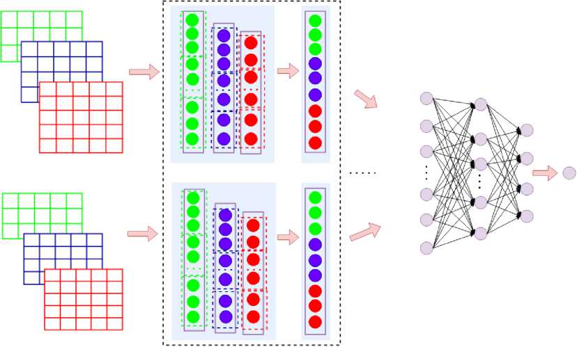
„    . .         ,                Dynamic chunk -based             _ ,    ,               Activation

Convolution operation                                .                Reshaped                 .   .

max pooling operation                                        function

Fig. 2. DCMP-CNN framework

• A.    Dynamic Chunk-based Max Pooling Method

To produce a new feature, the convolution kernel W £ R^kIi is employed for the performance of convolution operation. Then k refers to the convolution kernel window’s size. A feature c ™ is created from a window of words ⁷ i:i+k-1 ^by:

c ™ = f(W. 7^ —1 +Bi)                                  (5)

Here, the non-linear function is denoted by f, 7_l:l+k-1 is represented as the higher semantic segmentation and bias term is represented by Bi £ ^. Then the feature map is created by the convolution kernel W on the phrase ⁷ 1:k >⁷ 2:k+1 >⁷ 3:k+2 ■”>⁷ n-k+1:n with a window size of k:

Where, the arguments differ from one another in length n in this case, hence c ^m £ R^n-k+1 has various dimensions for various data. In the proposed framework, the selected tabular attributes are organized as ordered feature vectors so that the CNN can process them as one-dimensional structured sequences. This representation enables the convolution layers to capture local interactions among related variables such as age, BMI, smoking status, and regional information. By arranging the attributes in this structured form, the CNN can effectively learn meaningful relationships among the features before the pooling operation is applied. The pooling operation handles varying data lengths originally and catches the most significant feature for each feature map. Generally, CNN uses the max-pooling to gain the maximum value of c^m. However, the majority of the information in discourse arguments is lost such as the order of the patients. Guo et al. [18] introduced the concept of dynamic chunk-based max pooling operation as a means to partition an argument into multiple segments or chunks, based on the argument's length and the network's structure. Within this operation, the maximum value is selected from each chunk, facilitating the retention of essential information, such as the word order of the arguments. This dynamic chunk concept pertains to the segments derived from the feature map generated by the convolution layer, which is uniformly divided into “ck” segments. The calculation of the number of chunks, "ck" is determined dynamically by the Eq. (7). It's worth noting that if the feature "c m " is not evenly divisible by "ck" the last chunk will have a size equal to the modulus of the division.

ck = max

(ck.^11^]^)

Where, the top-most convolution layer’s fixed pooling parameter is called ck_top, TL is represented as the total number of layers in the CNN module, Cl is denoted as the current layer’s number and the data length is denoted by I. Map of features one argument is divided into equal chunk parts of c ^m , and we can extract the maximum value from each segment. The below Equations are used to select the essential features of each chunk.

c m = Chunkmax{[c ^m ,c ^m , -,c ^m_ _k +i ]}

, mm   m ck1>cck2> — ,cckn]

• B.    Improved Golden Eagle Optimization based CNN

In order to improve the performance of the CNN, the weights values are optimized using the IGEO approach. The proposed IGEO approach is a swarm-based metaheuristic algorithm, which is mostly used for global optimization issues. This optimization algorithm is created depending on the hunting GEs behaviours. This behaviour aims to highlight the mathematically designed exploration and application of the global optimization system. As natural representation of exploitation, transition, and exploitation from one to the other, the golden eagle strikes a clever balance between cruise, attack, and transition from one to the other. The process for weight optimization using GEO is described here;

Step 1: Initialization

First, initialize the GEO algorithm’s parameters. In this work, the weight f and bias l values of an IGEO-based CNN are used as the solutions. The following Equation shows the population of the solutions.

^ n = ^{7 i ,7 2 ,-,7 n ^}                                           (10)

Уп = К1Л..... f; l i ,l 2 .....U                                 (11)

Step 2: Fitness Function

After the initialization process, the fitness function is evaluated for each solution using the following Equation.

Fit_n = Maximum(Accuracy)

The Eq. (13) is utilized to calculate the accuracy value.

Accuracy =

TN+TP

TP+FP+TN+FN

Where, true positive and true negative values are denoted by TP and TN, and then false positive and false negative are represented by FP and FN.

According to the Eq. (12), the bias and weight values are selected as the CNN parameters with the maximum fitness or the ideal parameters. As a result, this strategy uses the position of the ideal solution to specify the location of the prey. The solution is modified based on the hunting behaviors of eagles, when the target fitness is not attained.

Step 3: Eagle’s spiral motion

Eagles hunt for prey by utilizing the spiraling motion. The best location is memorized by every golden eagle. At once, the eagle attracts both prey for searching the best food.

Step 4: Selection of prey

Each time, search agents choose a prey target from the collective memory. The attack and migration vectors of each golden eagle are found to be pertinent to its specific target. Moreover, in GEO the prey selection plays the most effective role.

Step 5: Exploitation

An attack can be planned by a golden eagle by employing a vector that begins at its current location and ends where it recalls the prey. The below Equation is utilized to evaluate the eagle attack vector (EA_V).

——?    ^ ,   ^

EAV = IQ - Kv

Where, K pl indicates that the eagle has found the best place for hunting prey. Eagle’s current location is denoted by

К .

Step 6: Exploration

The attack vector determines which cruise vector is used. Attack vectors are the opposite for cruise vectors, which are utilized for the circle. Finding the location of the deflection hyper plane is necessary before evaluating the cruise vector. Equation (15) provides the hyper-plane’s scale in n-dimensional space.

Th1k1 + Th2k2 +- + Thxkx = d ^ ZX=1 Thzkz = d(15)

d = Th.P(16)

Where, Th = [Th₁,Th₂, ...,Th_X] is represented as the normal vector. P = [P₁,P₂, .,P_X] is a random vector. Then the cruise vector is determined as follows:

cV = ^x=i azkz = ^x=i c^kz(17)

Where, EA_V = [a₁, a₂,..., a_x] is the eagle attack vector and К = [k₁, k₂, ..., k_x] is denoted as the variable vector. Then К * = [k 1 , k₂, ., k X ] is a selected prey’s location.

The following procedure is used to obtain the randomly generated n-dimensional target point C on the cruise hyper-plane for the golden eagle i.

Step 1: Out of all the variables, one is randomly selected as the best one.

Step 2: The random parameters are fixed to absolute variables while taking the X^th variable into consideration.

Step 3: The parameter of the set parameter is calculated using the following Equation (18).

^z^                       (18)

'

Where, e_r is the terminal point and d represents the RHS value of Equation (18).

Step 4: Updating the position

The attack vector and the cruise vector are the two kinds of movements in GEs. The below Equations are used to update the position in t iteration.

f2L

Akv = randJAt     + ran^ci^-.(19)

ll^AvilH

ИМИ = ЛЯ^ and WcvW = XY^(21)

Then the golden eagle’s position t + 1 is,

K^{t +1} = k ^t + Ak V

if Fit ^new > Fit^M memory updated otherwise      memory intact

Step 5: Exploration to Exploitation

In GEO, P_a and P_e are utilised to transition from exploitation to exploration.

Pa =Pa+ — [Pa - Pa](24)

a     a   Mt a     алV /

P =Pt+ — [Pf - Pt](25)

e     e    Mt L e

Where, the starting and final propensity cruise is represented by P f and P f . Then P a and P ^ are represented as the first and last propensity attack, greatest iteration is denoted by Mt and t is the current iteration.

4.    Experimental Results

The dataset description, experimental setup and results are detailed in this section.

• 4.1.    Dataset Description

  This paper utilizes a medical dataset from the Kaggle repository for medical insurance cost prediction. The dataset is presented in https://www.kaggle.com/code/subhakarks/medical-insurance-cost-analysis-and-prediction. It contains 1338 records and every record has a person’s specific data such as BMI, children, sex, region, smoker, charges and age. Although the dataset contains only 1338 samples with a limited number of features, it is a widely used benchmark dataset for evaluating healthcare cost prediction models. The objective of this work is not to apply deep learning only to large scale datasets but to investigate whether optimized deep learning frameworks can effectively capture nonlinear relationships among demographic and lifestyle attributes. In this study, the CNN architecture is utilized to learn feature interactions among variables such as age, BMI, smoking status, and regional factors, while the BFHO feature selection method reduces redundant attributes and the IGEO optimization algorithm improves parameter learning. This combination helps enhance prediction performance and learning stability even when the dataset size is relatively small. Moreover, the dataset description is detailed in Table 1.

• 4.2.    Experimental Results

  The proposed prediction model is simulated on a computer operating Windows 10 OS, featuring an Intel Core i3 CPU and 4 GB of memory with Matlab 2020a installed. The prediction performance of the proposed approach is compared with other traditional approaches like Improved Whale Optimization Algorithm (IWOA), FHO, Improved Manta Ray Foraging Optimization (IMRFO), Honey Badger Algorithm (HBA), and Binary Grey Wolf Optimizer (BGWO). All experiments were conducted with controlled initialization settings using a fixed random seed to ensure reproducibility. Each model was executed for multiple independent runs and the reported results correspond to the average performance obtained across these runs to minimize randomness in the optimization process. Hyperparameters of the CNN architecture and optimization algorithms were determined through systematic empirical tuning using validation data. The BFHO and IGEO optimization procedures were terminated when the maximum number of iterations was reached or when the improvement in the fitness value between successive iterations became negligible, indicating convergence. In addition, all compared models were trained under identical experimental conditions including the same number of epochs, training data partitions, and stopping criteria to ensure a fair comparison of training time and prediction performance under the available computational environment.

Table 1. Dataset description

Name of the feature	Explanation	Value
BMI	Weights that are abnormally high or low in relation to height can help us understand the human body	Average value- 18.5-24.9
Children	No. of children	Integer
Sex	Persons Gender	Female = 0, Male= 1
Region	Location of the person	NE = 0, NW = 1, SE = 2, SW= 3
Smoker	State of smoking	No= 1, Yes= 0
Charges	Medical ills	Integer
Age	Persons age	Integer

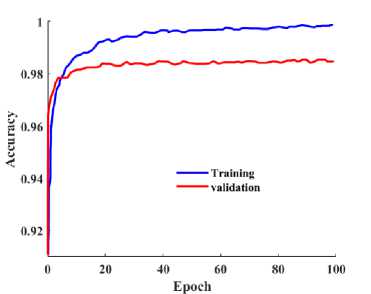
Fig. 3. Accuracy of training and validation curve

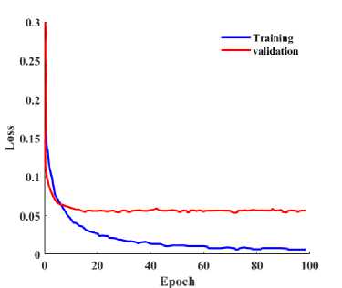
Fig. 3 shows the performance of accuracy in the validation and training curve. The accuracy value should be high for the improved performance. While increasing the epoch values, the validation and training curves’ accuracy are also increasing. Comparing the training and validation curve, the training curve has the better performance in accuracy. Fig. 4 shows the performance of training loss and validation loss curve. For both the validation and training curves, the loss decreases with increase in the epochs. The training curve has very small loss compared to the validation curve.

• Fig. 4.    Loss of training and validation curve

• Fig. 5.    Comparison of fitness value

• Fig. 6.    Number of selected features

Training Time(seconds)

Fig. 7. Comparison of the training time

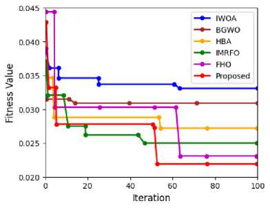
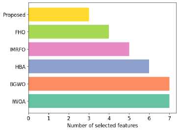
The comparison of the fitness values is displayed in Fig. 5. The proposed approaches’ fitness function is compared with the existing approaches like FHO, IMRFO, HBA, BGWO and IWOA. From the experimental result, the proposed approach has a better fitness value than the existing approaches. Then Fig. 6 shows the number of selected features for the proposed and existing optimization algorithms. Based on the outcome, it is evident that the proposed model has significantly decreased the number of selected features. It retained only the most relevant features, those that directly impacted the results, while discarding the rest. The model's selection process resulted in fewer than half of the total features within the dataset being chosen. From the findings it is found that the proposed BFHO stands out as the most effective feature selection method.

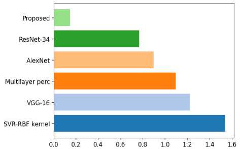
The proposed method’s training time is compared with the other deep learning methods such as ResNet-34, AlexNet, Multilayer perc, VGG-16 and SVR-RBF kernel that is shown in Fig. 7. The proposed model takes much less training time for error prediction compared to the existing methods. This is because the proposed DL approach contains the less parameters and low complexity. Then the overall performance of the DL models in terms of RMSE, R2_score training and testing values and the cross validation values is detailed in Table 2. In this study, insurance cost prediction is formulated as a regression problem because the target variable (medical charges) is continuous. Therefore, the final model performance is evaluated using regression metrics such as RMSE, R² score, cross validation score, and MAPE, which are appropriate for continuous value prediction. The accuracy related indicators such as TP, TN, FP, and FN mentioned in the optimization stage are not used for the final regression evaluation but are incorporated internally within the IGEO fitness calculation to guide the optimization process during model training. These indicators are derived by temporarily discretizing prediction outcomes to assess optimization convergence behavior. However, the final performance assessment and comparison of the proposed model with other methods strictly rely on regression based metrics to ensure statistical consistency with the insurance cost prediction task. The RMSE shows the prediction quality. RMSE measures the average magnitude of prediction error between the actual and predicted insurance charges, while the R² score evaluates how well the model explains the variance in the target variable. The cross validation score reflects the generalization capability of the model across different data partitions, and MAPE quantifies the percentage deviation between predicted and actual cost values. The fitness value is utilized within the optimization stage to guide feature selection and parameter tuning. Therefore, the RMSE value is interpreted relative to the scale and distribution of the insurance charge values in the dataset rather than using a fixed universal threshold. In Table 2, the RMSE values of all DL models are shown in the above mentioned range. However, compare to the all models, the proposed method’s RMSE value 0.33362 is a better value, so it gives a more exact prediction than the other five DL models. Furthermore, the higher score of R2 is better and it usually ranges from 0 to 1. Hence the proposed DL approach contains both training and testing values of R2 that are very high compared to the all DL approaches. One statistical technique for estimating the accuracy of deep learning models is cross-validation. And also, it is utilized to prevent the over fitting. If the cross-validation score is higher, then the model is better to generalize the unseen data. In this Table, compare to the existing methods, the proposed technique gives the high cross-validation score that is 0.853492, so it is the best model for generalizing the unseen data. To further validate the generalization capability of the proposed model and address potential overfitting concerns, additional diagnostic observations were conducted during the training process. The learning behavior of the model was monitored through training and validation curves across epochs, as illustrated in Fig. 3 and Fig. 4. The curves demonstrate consistent convergence patterns without significant divergence between training and validation performance, indicating stable learning. Furthermore, the model evaluation was performed using cross validation across multiple data partitions, and the resulting scores showed limited variance, confirming that the model maintains stable performance across different folds. The dropout analysis presented in Table 4 also supports the regularization capability of the model, where the optimal dropout rate of 0.5 achieved the lowest MAPE value of 1.54, while the absence of dropout resulted in higher prediction error. These observations collectively provide empirical evidence that the proposed IGEO optimized CNN framework improves generalization performance while mitigating the risk of overfitting.

Table 2. DL models outcomes

Model	RMSE	R2_score (training)	R2_score (test)	Cross-validation
SVR-RBF kernel	0.479808	0.741410	0.782694	0.744528
VGG-16	0.465206	0.741150	0.783800	0.825999
Multilayer perc	0.358771	0.847234	0.871283	0.842307
AlexNet	0.409725	0.74636	0.794312	0.755814
ResNet-34	0.362509	0.831859	0.853683	0.823654
Proposed	0.333362	0.860118	0.883213	0.853492

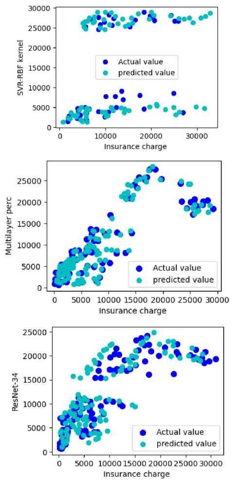
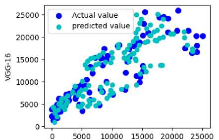
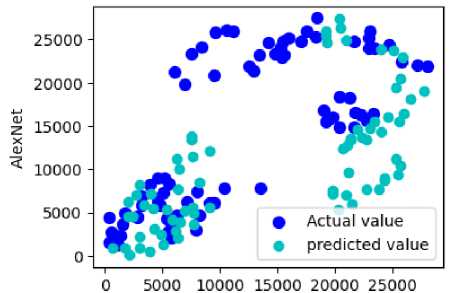
Fig. 8. The actual and predicted values are each DL methods. a) SVR-RBF kernel, b) VGG-16, c) Multilayer perc, d) AlexNet, e) ResNet-34 and f) Proposed technique

Insurance charge

Insurance charge

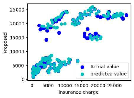
Fig. 8 shows the existing and proposed deep learning techniques actual and predicted values in the form of scatter plots. Moreover, the dots are used in scatter plots to symbolize values for two distinct numerical variables. Compared to the all six DL approaches, the proposed method only gives the accurate prediction that is shown in Fig. 8.

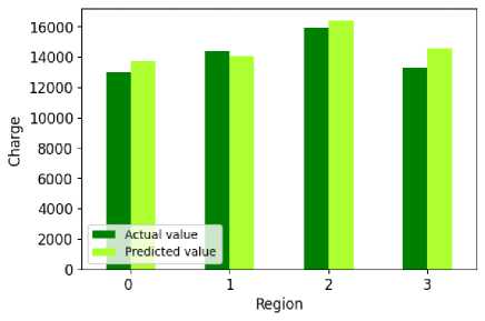
Fig. 9. Region vs insurance charges

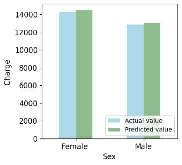
Fig. 10. Gender vs insurance charges

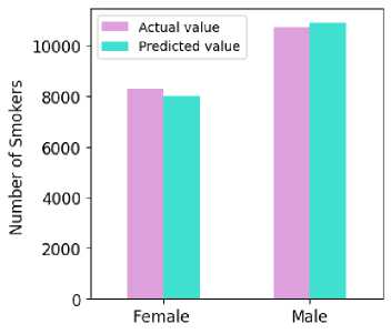
Fig. 11(a). Performance of the smokers amount

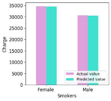
Fig. 11(b). Smokers vs insurance charges

The visualizations shown in Fig. 9 - Fig. 11 are presented primarily for exploratory data analysis to illustrate observable trends in insurance charges across region, gender, and smoking attributes. These graphical observations are descriptive and do not imply causal socio-economic relationships. To avoid speculative interpretation, statistical hypothesis testing was conducted to verify whether the differences among these demographic groups are statistically significant. The results of these statistical tests are summarized in Table 6, which provides a more rigorous analytical validation of the observed patterns. As Fig. 9 illustrates, the performance of the insurance costs differs depending on the location and it also shows the difference between the predicted and actual values. In comparison to other regions, the southeast has higher health insurance costs. Moreover, compared to the actual and predicted values, the predicted values are almost nearer to the actual values. Fig. 10 demonstrates that the medical insurance costs for women are consistently higher than those for men. The statistic shows that the insurance actual costs for a female are $14,000, while the costs for a guy are approximately $13,000. Moreover, the insurance prediction costs are approximately $13,500 for a male and $14,100 for a girl. Comparing both predicted and actual values, the predicted value is almost the same as the actual value.

Table 3. The effect of the quantity of blocks and filters in CNNs on the cost prediction MAPE performance

Number of blocks	Numbers of filters	MAPE
1	16	6.14
1	32	5.35
1	64	4.02
1	128	4.38
1	256	4.63
2	16,8	4.27
2	32,16	2.61
2	64,32	2.52
2	128,64	2.55
2	256,128	4.48
3	32,16,8	3.06
3	64,32,16	2.19
3	128,64,32	1.42
3	256,128,64	3.13
3	512,256,128	4.65
4	64,32,16,8	3.28
4	128,64,32,16	3.02
4	256,128,64,32	4.16
4	512,256,128,64	4.67
5	128,64,32,16,8	3.39
5	256,128,64,32,16	4.64
5	512,256,128,64,32	5.13

Table 3 presents the variation in the number of blocks and the quantity of filters within DCMP-CNN on the Mean Absolute Percentage Error (MAPE) performance for insurance prediction. Number of blocks represents the number of building blocks in the CNN architecture. Each block typically consists of convolutional and pooling layers. Increasing the number of blocks can introduce additional layers for feature extraction and potentially capture more complex patterns in the data. Numbers of filters indicate the quantity of filters (also known as kernels) employed in each block of the CNN. Filters are responsible for extracting features from the input data. More filters can help the network capture a broader range of features. Values separated by commas represent the number of filters in different layers within the same block. MAPE is a metric used to evaluate the accuracy of cost predictions. It quantifies the percentage difference between predicted and actual cost values. Lower MAPE values indicate more accurate predictions. As observed in the table, different configurations yield varying MAPE values. Configurations with one block and a low number of filters ("1 16") result in higher MAPE values, suggesting less accurate predictions. Conversely, configurations with more blocks and filters ("3 128,64,32") produce lower MAPE values, indicating improved predictive accuracy. The table thus offers a comprehensive analysis of how the CNN architecture's structure, specifically the number of blocks and filters, affects the model's ability to predict healthcare costs accurately. Researchers can use this information to select the most suitable architecture for their specific cost prediction tasks.

Table 4. Utilizing CNNs for cost prediction, the MAPE of various dropout rates

Dropout Rate	MAPE
0.75	3.78
0.5	1.54
0.25	2.53
0.15	3.65
0	5.02

Table 4 evaluates the impact of different dropout rates on the performance of CNNs in health insurance cost prediction. Each row represents a specific dropout rate, and the corresponding MAPE value indicates the level of prediction accuracy achieved at that rate. A dropout rate of 0.5 results in the lowest MAPE of 1.54, indicating the most accurate cost predictions. As the dropout rate increases or decreases from 0.5, the MAPE values vary with higher dropout rates like 0.75 and 0.15, which yield less accurate predictions with MAPE values of 3.78 and 3.65, respectively. Especially, a dropout rate of 0 (no dropout) leads to the highest MAPE of 5.02, suggesting the least accurate predictions and potential overfitting. Thus, the table describes how different dropout rates influence the accuracy of cost predictions when utilizing CNNs. It serves as a reference for selecting the most appropriate dropout rate to achieve optimal predictive performance in health insurance cost prediction tasks in the proposed approach.

Table 5. The MAPE of each activation function in a CNN used to predict costs

Activation Function	MAPE
LReLU	1.47
ReLU	1.54
Sigmoid	3.45
Tanh	5.22

Table 5 presents the MAPE values obtained by employing different activation functions in the proposed insurance prediction model. Specifically, each activation function was simultaneously applied to both the convolutional and fully connected layers of the model. The output layers of each model utilized a consistent softmax classifier for the prediction. Sigmoid and Tanh activation functions yield higher MAPE values of 3.45 and 5.22, respectively. These higher MAPE values suggest less accurate insurance cost predictions with these activation functions. LReLU (Leaky Rectified Linear Unit) and ReLU (Rectified Linear Unit) activation functions result in the lowest MAPE values of 1.47 and 1.54, respectively, indicating highly accurate insurance cost predictions. Thus, selecting the most suitable activation function to achieve optimal predictive performance in insurance cost prediction tasks, with LReLU and ReLU appear as favorable choices based on the lowest MAPE values.

Table 6. Statistical significance testing of prediction performance

Model	Mean RMSE	Std. Deviation	95% Confidence Interval	p-value (vs Proposed)
SVR-RBF kernel	0.4798	0.021	0.438 – 0.521	<0.01
VGG-16	0.4652	0.019	0.428 – 0.502	<0.01
Multilayer Perceptron	0.3588	0.015	0.329 – 0.388	0.032
AlexNet	0.4097	0.017	0.376 – 0.443	<0.01
ResNet-34	0.3625	0.014	0.335 – 0.389	0.041
Proposed IGEO-CNN	0.3333	0.011	0.311 – 0.355	—

Table 6 presents the statistical significance analysis of prediction performance for the proposed IGEO-CNN model and the baseline models using RMSE as the evaluation metric. The mean RMSE represents the average prediction error obtained across multiple experimental runs, while the standard deviation indicates the variability of model performance. Lower standard deviation values imply more stable and consistent predictions. The 95% confidence interval provides the expected range within which the true mean RMSE of each model lies with high probability. The proposed IGEO-CNN model achieves the lowest mean RMSE of 0.3333 with the smallest standard deviation of 0.011, indicating superior accuracy and stability. The p-values obtained from paired statistical tests compare each baseline model with the proposed approach. Since all p-values are below the 0.05 significance threshold, the improvements achieved by the proposed model are statistically significant. This confirms that the superior performance of the IGEO-CNN model is not due to random variation but reflects a meaningful improvement over existing methods.

5.    Conclusion

Deep learning (DL) is one of the strongest techniques that can use a variety of applications and systems to tackle a variety of problems. In the healthcare industry, predicting medical insurance costs is a challenge that requires research and improvement. In this paper, the deep learning algorithms are utilized to predict the cost of medical insurance. First, the pre-processing is done by using the Z-score method. Then the meta-heuristic optimization algorithm modified FHO is proposed for the feature selection. This proposed feature selection approach is used to select the best features from the medical dataset. Then the deep learning classifier improved CNN is utilized to predict the error rate from the selected features. Furthermore, DCMP and IGEO are the two techniques that are utilized to improve the CNN network. The medical dataset is utilized in this article for training and testing the proposed model. From the experimentation it is found that the proposed approach's fitness function, when compared to conventional techniques such as FHO, IMRFO, HBA, BGWO, and IWOA, consistently outperforms with a significantly better fitness value. Future work will explore the broader applicability and potential challenges of neural networks in modeling various patient outcomes and trajectories using high-dimensional electronic health records, focusing on interpretability and generalizability.

All the Declarations and StatementsAuthor Contributions Statement

P. Sherly Kanaga Priya: Data Curation and Software Implementation: Handled data acquisition, dataset preprocessing, and implementing the research model; Formal Analysis, Visualization, and Statistical Analysis: Performed in-depth analysis of experimental results, prepared performance charts, and ensured the statistical robustness of the evaluation; Writing – Drafted the initial manuscript, contributed to the literature survey, and documented the technical background of the study.

G. Uma Maheswari: Conceptualization, Methodology, and Supervision: Proposed research ideas, Constructed the overall framework, and supervised project execution; Writing – Review and Editing, and Project Management: Reviewed and edited the manuscript, ensured clarity and coherence, and helped coordinate project milestones and deadlines.

All authors have read and agreed to the published version of the manuscript.

Conflict of Interest Statement

The authors declare no conflicts of interest.

Funding Declaration

The authors received no financial support for the research, authorship, and/or publication of this article.

Data Availability Statement

The data used in this study are available from the corresponding author upon reasonable request.

Ethical Declarations

This research did not involve human subjects or animals. Therefore, no statements of ethical approval are required.

Acknowledgments

We sincerely thank the experts for their professional evaluation and valuable recommendations, which have contributed to improving the quality of this manuscript.

Declaration of Generative AI in Scholarly Writing

No generative AI or AI-assisted technologies were used in the preparation of this manuscript.

Abbreviations

The following abbreviations are used in this manuscript:

FS - Feature Selection

DCMP - Dynamic Chunk-based Max Pooling

IGEO - Improved Golden Eagle Optimization

CNNs – Convolutional Neural Networks

IWOA - Whale Optimization Algorithm

FHO - Fire Hawk Optimization

IMRFO - Improved Manta Ray Foraging Optimization

HBA - Honey Badger Algorithm

BGWO - Binary Grey Wolf Optimizer

ML - Machine learning

ACO - Ant Colony Optimization

GA - Genetic Algorithm

WOA - Wolf Optimization Algorithm

PSO - Particle Swarm Optimization

EOBL - Elite Opposition-Based Learning

Appendix

None.