Enhanced Dynamic Algorithm of Genome Sequence Alignments

Published Online May 2014 in MECS

In bioinformatics, a sequence alignment is a way of arranging the primary sequences of Deoxyribonucleic acid (DNA) such as expressed sequence tags, Ribonucleic acid (RNA), or protein to identify regions of similarity. This similarity may be a consequence of functional, structural, or evolutionary relationships between the sequences. This field includes components of mathematics, biology, chemistry, and computer science. Bioinformatics means the analysis of biological information using computers and statistical techniques, Bioinformatics is the tools for analysis of Biological Data as shown in Figure 1 [1].

Aligning two long DNA sequences requires a long time on a single processor and a very large memory capacity [2]. Aligned sequences of nucleotides or amino acids residues are typically represented as rows within a matrix. Gaps are inserted between the residues so that identical or similar characters are aligned in successive columns [3]. There is a lot of sequence alignment algorithms such as dynamic algorithms and heuristic algorithms. Dynamic algorithm includes many algorithms for example Needleman-Wunsch and Smith-Waterman [3]. The heuristic algorithm includes Basic Local Alignment Search Tools (BLAST) and FASTA.

Sequence is an ordered list of objects or events like a set, it contains members that called elements or terms, and the number of terms is called the length of the sequence [4]. Computational biology involves the development and application of data-analytical and theoretical methods, mathematical modeling and computational simulation techniques to the study of biological, behavioral, and social systems [5]. The problem in sequence alignment is the execution time is very high and a modified algorithm is introduced to minimize that time. So the execution time becomes lower and the efficiency is high. There are two approaches to make the sequence alignments as explained in the following.

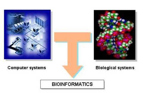
Fig. 1. Bioinformatics basics

• A.    Global Alignment

Global alignment assumes that the two proteins are basically similar over the entire length of one another. The alignment attempts to match them to each other from end to end, even though parts of the alignment are not very convincing [6], [7].

NLGPSTKDFGKISESREFDNQ I          Illi I

QLNQLERSFGKINMRLEDALV

• B.    Local Alignment

Local alignment searches for segments of the two sequences that match well. There is no attempt to force entire sequences into an alignment, just those parts that appear to have good similarity, according to some criterion are considered. Using the same sequences as above, Local alignment becomes as follow:

NLGPSTKDDFGKILGPSTKDDQ

Illi

QNQLERSSNFGKINQLERSSNN

Most commonly used algorithm for local alignment is Smith-Waterman algorithm global alignment, which is the best as it gets a maximum match between the sequences. These two types of alignment are used to make a comparison between genetic sequences like Expressed Sequence Tags (ESTs). ESTs are small pieces of DNA sequence (usually 200 to 500 nucleotides long) that are generated by sequencing either one or both ends of an expressed gene. They are short DNA molecules reverse-transcribed from a cellular mRNA population [8], [9].

The organization of the remaining paper is as follows: Section 2 presents an overview about bioinformatics algorithms in the previous works. Section 3 presents the proposed algorithm. Section 4 presents the experimental results. Finally, the conclusion is illustrated in section 5.

• II.  Related Work

The short or similar sequences can be aligned by using the hand. However, most interesting problems require the alignment of sequence length. The Pair-wise algorithm used to compare the two sequences. The following example illustrates an alignment between the sequences      A=.ACAAGACAGCGT      and

B=.AGAACAAGGCGT [3].

A = ACAAGACAG-CGT

I II I II III

В = AGAACA-AGGCGT

• Fig. 2. Alignment of two sequences

The objective is to match identical subsequences as far as possible. In the example, nine matches are highlighted with vertical bars. However, if the sequences are not identical, mismatches are likely to occur as different letters are aligned together. Two mismatches can be identified as shown in the example: a C of A aligned with a G of B, and a G of A aligned with a C of B. The insertion of spaces produced gaps in the sequences. They were important to allow a good alignment between the last three characters of both sequences. An alignment can be seen as a way of transforming one sequence into the other. From this point of view, a mismatch is regarded as a substitution of characters. A gap in the first sequence is considered an insertion of a character from the second sequence into the first one, whereas a gap in the second sequence is considered a deletion of a character of the first sequence. In the previous example, A can be converted into B in four steps:

• 1)    Substitute the first C for a G;

• 2)    Substitute the first G for a C;

• 3)    Delete the second C; and

• 4)    Insert a G before the last three characters.

Once the alignment is produced, a score can be assigned to each pair of aligned letters, which called aligned pair according to a chosen scoring scheme. We usually reward matches and penalize mismatches and gaps. The overall score of the alignment can then be computed by adding up the score of each pair of letters. For instance, using a scoring scheme that gives a +1 value to matches and -1 to mismatches and gaps, the alignment of Figure 2 score equals 9 * (1) + 2 * (-1) + 2 * (-1) = 5. The similarity of two sequences can be defined as the best score among all possible alignments between them. Note that it depends on the choice of scoring scheme. Next section introduces the multiple algorithms that used for this comparison.

Actually all the previous works of dynamic sequences alignments depend on Needleman-Wunsch, Smith– Waterman, and longest common subsequence algorithms, and the contributions of these works falls on how to speed up and reduced the memory space that used in these algorithms. In [2] is developed a parallel solution to achieve the optimum alignment with relatively good performance. The shared memory parallel architecture is the focus of this work therefore; it have considered off-the-shelf systems like multi-core CPUs as well as advanced shared memory platforms.

The work in [4] is proposed a solution that utilizes both shared and distributed memory architectures via cloud technology to enhance the performance of evaluating the statistical significance for pair of DNA sequences. Therefore, the restriction on the sequence sizes is released to be in megabyte-scale, which was not supported before for the statistical significance problem.

A Needleman-Wunsch Algorithm

The standard global alignment algorithm is referred to as Needleman-Wunsch algorithm [10]. This algorithm computes the similarity between the two sequences A and B of lengths m and n, respectively, using a dynamic programming approach. Dynamic programming is a strategy of building a solution gradually using simple recurrences [7]. The key observation for the alignment problem is that the similarity between sequences A[1..m] and B[1..n] can be computed by taking the maximum of the three following values:

• •    The similarity of A [1……m -1] and B [1…….n -1] plus the score of substituting A[m] for B[n];

• •    The similarity of A [1……m -1] and B [1……n] plus the score of deleting aligning A[m];

• •    The similarity of A [1……m] and B [1……n -1] plus the score of inserting B[n].

From this observation, the following recurrence can be derived by:

sim ( A[1..i], B[1..j] ) = max { sim ( A[1..i -1], B[1..j

• - 1] ) + sub ( A[i], B[j] ); sim ( A[1..i -1], B[1..j] ) + del ( A[i] ); sim ( A[1..i], B[1..j -1] ) + ins ( B[j] )}   (1)

Where sim (A, B) is a function that gives the similarity of two sequences A and B, and sub (a, b), del (c) and ins (c) are scoring functions that give the score of a substitution of character a for character b. where del (c) and ins (c) are deletion of character c, and an insertion of character c, respectively. This recurrence is complete with the following case:

sim ( A[0], B[0] ) = 0; where A[0] and B[0] are defined as empty strings. To solve the problem with this recurrence, the algorithm build an (m +1) × (n +1) matrix M where each M [i, j] represents the similarity between sequences A [1....i] and B [1….j] as shown in Figure 3. The first row and the first column represent alignments of one sequence with spaces. M [0, 0] represents the alignment of two empty strings, and is set to zero. All other entries are computed with the following formula:

M [i, j] = max {M [i -1, j -1] + sub (A[i], B[j]);

M [i -1, j] + del (A[i] ); M [i, j -1] + ins ( B[j])}      (2)

The matrix can be computed either row by row from left to right or column by column (from top to bottom. In the end, M [m, n] will contain the similarity score of the two sequences. Since there are (m+1)*(n+1) positions to compute and each one take a constant amount of work. This algorithm has time complexity of O (n2). Clearly, it has also quadratic space complexity since it needs to keep the entire matrix in memory.

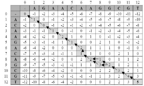
Fig. 3. Dynamic programming matrix for the global alignment

Figure 3 shows the standard dynamic programming matrix for the global alignment of sequence A=ACAAGACAGCGT and B=AGAACAAGGCGT with paths to retrieve optimal alignments indicated with arrows. Once the matrix has been computed, the actual alignment can be retrieved by tracing a path in the matrix from the last position to the first. The trace is a simple procedure that compares the value at each M [i, j] to the values of its left, top and diagonal entries according to the formula that given above. For instance, if M [i, j] = M [i, j -1] + ins (B[j]), the trace reports an insertion of character B[j] and proceeds to entry M[i, j -1]. Alternatively, pointers can be saved on each entry during the computation of the matrix so that this evaluation step can be avoided at the cost of more memory usage. Since the path can be as long as O (m + n), this procedure has linear time complexity. Note that sometimes more than one path can be traversed and as a result multiple high-scoring alignments can be produced. In the matrix of Figure 3, two optimal alignments can be retrieved as shown in Figure 2 and Figure 4.

A = ACAAGACA-GCGT

I II I I Illi

В = AGAACA-AGGCGT

Fig. 4. Optimal alignment retrievable from the matrix of Fig.3

It is often useful to see the dynamic programming solution for the sequence alignment problem as a directed weighted graph with (n +1) × (m +1) nodes representing each entry (i, j) of the matrix, and having the following edges:

• •    ((i -1, j -1), (i, j)) with weight equals to sub ( A[i], B[j] );

• •    ((i -1, j), (i, j)) with weight equals to del ( A[i] );

• •    ((i, j -1), (i, j)) with weight equals to ins ( B[j] );

A path from node (0, 0) to (n, m) in the alignment graph corresponds to an alignment between the two sequences, and the problem of retrieving an optimal alignment is converted to the problem of finding a path in the graph with highest weight.

• B.    Smith-waterman algorithm:

The Smith–Waterman algorithm compares segments of all possible lengths and optimizes the similarity measure. It has the desirable to find the optimal local alignment with respect to the scoring system. The main difference between Smith-Waterman and Needleman is adding the possibility of zero value to the main function of Needleman algorithm [11],[12]. The formula for computing M (i, j) in (2) becomes:

M (i, j) = MAX{ 0;M (i-1, j-1) + sub (A(i), B(j));

M(i-1,j) + del(A(i)); M(i,j-1) +ins (B(j))}

Initialization:

Gap=0, Match=+1, Mismatch=-1,

Assume the sequence A=GCCCTAGCG, and B = GCGCCAATG. Figure 4 shows the optimal local alignment that get from running the smithwaterman code as follows:

• -    A = GCCCTAGCG

GCG

• -    B =       GCGCCAATG

The score of smith alignment=(3*1)+(0*-1)+(0*0) =3

• C.    longest common subsequence problem:

The longest common subsequence (LCS) problem is the third application of dynamic programming and used to find the longest common subsequence to all sequences in a set of sequences [13]. It is considered to fill in a cell the three values V1, V2, and V3 that shown as follows:

• - V1 = the value in the cell to the left

• - V2 = the value in the cell above

• - V3 = the value in the cell to the above-left

The main function in the LCS strategy: Max = {V1, V2, V3+1} if C1 equals C2, V3 if C1 is not equal to C2, where C1 is the character above the current cell and C2 is the character to the left of the current cell.

Termination: It is adding arrows that point pack to get the value for the current cell and these arrows are used in the tracing back.

Tracing back to find an actual LCS:

In the tracing back step it uses the cell pointers that we draw. When you have a pointer to the above-left cell, the value in the current cell is equal 1 and it is more than the value of the above-left cell. This means that the characters to the left and above are equal (match) else the characters are not equal (mismatch) or gaps as shown in Figure 4.

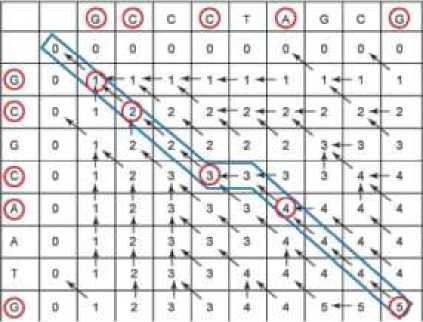
Fig. 4. Shows the best matches in LCS matrix with trace back and matches [13].

From the trace back:

It is found the score of LCS alignment = 5.

Performance: time Complexity is O (M*N) as it is need to fill all the cells in the matrix, and time of backing trace is (M+N).

• III.    The Proposed Algorithm

The proposed algorithm is a modified of global dynamic algorithm, where it is depend on filling the three main diagonals without filling the entire matrix by the unused data as shown above in the pervious work section. To explain the modified algorithm by given two sequences A and B, and create a matrix M×N where M is the length of first sequence, N the length of second sequence. Every non-decreasing path from (0, 0) to (M, N) corresponds to a global alignment of the two sequences. There are five main steps for the EDAGSA algorithm as follow:

Step1: Initialization

Gap= -1

Match= +1

Mismatch= -1

C (0, 0) = 0

C (0, 1) = C (0, 0) + Gap

C ( j , 0) = C (0, 0) + Gap

Step2: Detect the three main diagonals in the matrix.

Step 3: Main Iteration

For each cell in the three main diagonals:

For each i = 1 . . . M

For each j = 1 . . . N if ( i = j )

C ( i , j ) = (C ( i - 1, j - 1) + match)

Dir (i, j) = (DIAG)

if ( i ≠ j )

C (i, j) = max

{C ( i - 1, j - 1) + mismatch, case 1

C ( i - 1, j ) + gap, case2

C ( i , j - 1) + gap, case3}

Hint: the three values in the maximum function needn’t be found it must be at least one value.

dir ( i , j ) =

{DIAG, if case 1

LEFT, if case 2

UP, if case 3}

Step 4: Termination

C ( M , N ) is the optimal score, and from dir ( M , N ), we can trace back the optimal alignment.

Step 5: Performance

Time: O (3 M + 1) if the 2 sequence have same length or O (3 M + 2) if the 2 sequence have different length.

Space: O (3 M + 1) if the 2 sequence have same length or O (3 M + 2) if the 2 sequence have different length.

• A. EDAGSA Case Study

Given two sequences A=“ACAAGACAGCGT” and B=“AGAACAAGGCGT”

Create a matrix of size M*N. The main steps of

EDAGSA algorithm is as follow:-

Step1: Initialization

Gap=-1

Match=+1

Mismatch=-1

dir = the direction of the trace back for optimal alignment.

C(0, 0) = 0

C(0, 1) = C(0,0)+Gap

= -1

F(j, 0) = C(0,0) +Gap = -1

Step2: Detect the three main diagonals in the matrix.

Step3: Main Iteration

Calculate the values for each cell in the three main diagonals as shown in Table1:

C[1,1]=C[0,0]+match=0+1=1     (i=j)

dir = diagonal

C[1,2]= max(C[0,1],C[1,1],C[0,2]) +mismatch (i≠j)

C[0,2] not have any value so

C[1,2]=max(C[0,1],C[1,1]) +mismatch

= max(-1,1)+(-1)=1-1=0

dir = the maximum value = left

And so on for all the 3 diagonal values, the matrix will be as follow as shown in table1.

Step4: Termination

C[M,N] is the optimal score

The optimal score is 5 and trace back the optimal alignment from this optimal score position by the dir value, thus the optimal alignment is shown below in the bold characters.

A G AA G A C A - GCGT

A C AA C A - A G GCGT

The Score is equal (9)*1+ (2)*-1+(2)*-1= 9-2-2 = 5

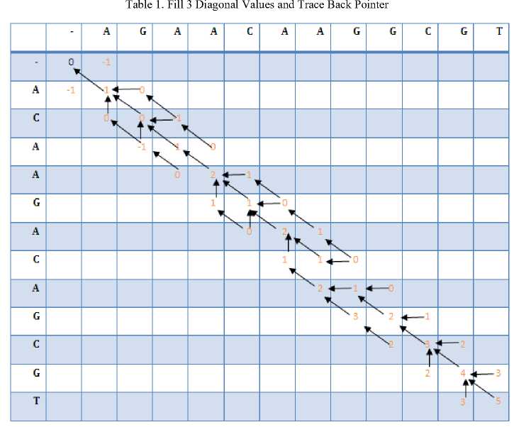
Step5: Performance

Time = O(3*M+1) = O(37) where M = 12 and space = O(3*12+1) = O(37)

From the last matrix we found that EDAGSA algorithm find the same optimal solution as dynamic programming matrix for the global alignment. Also it can be used for the longest common subsequence algorithm. EDAGSA ignored the most unused data of the matrix, and therefore it reduces the execution time for the alignment and increase the performance.

• IV.    Experimental result

  To verify EDAGSA algorithm the experimental results are done for the comparison between EDAGSA and the traditional algorithms such as fast longest common subsequences LCS, Needleman-Wunsch Algorithm, and Smith-Waterman when the sequences is A= GCCCTAGCG and B= GCCCAATG.. It is found the execution time for the alignment by using Needleman-Wunsch algorithm is = 0.7929783 msec, and it =

  0.5368433 msec by the Smith-Waterman algorithm, and longest common subsequences algorithm is =0.4060487 msec, and finally = 0.2605421 msec by EDAGSA

algorithm.. From these values we found that our algorithms EDAGSA achieve the least execution time and this come from ignoring the unused data of the matrix and evaluate the only three main diagonals.

The four dynamic algorithms are applied on the two types of human insulin such as EST'S sequence1 with accession number: C07137.1 and EST'S sequence2 with accession number: C07145.1 with length 231, then it found the total execution time for the alignment by using Needleman-Wunsch algorithm is 4.4839166 millisecond, and it = 4.3071470 millisecond by the Smith-Waterman algorithm, and Longest Common Subsequences algorithm is = 3.0585219 millisecond, and finally= 2.2647422 millisecond by EDAGSA algorithm. Also, from these values we found that our algorithms EDAGSA achieve the least execution time.

For multi-sequences alignments the previous work in the bioinformatics algorithms depend on making a comparison in files and this take more time. Also this work suggests for multi-sequences alignments to make the comparison in a database rather than on files, which will speed the execution time of the comparison.

The GUI interface for the proposed algorithm is introduced in Figure 5. In Figure 6 the frame that compare the input sequence with the sequences in data base to identify which one in the data base is mot similar, then the best score is returned and the sequence in the data base that achieve most score as shown in Figure 7. In data base we set a DNA sequences to make comparison between them to identify the big similarity between them.

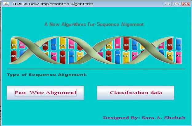
Fig. 5 . The GUI of Two Sequence Alignment

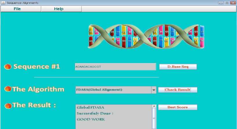
Fig. 6. The alignment of the sequences

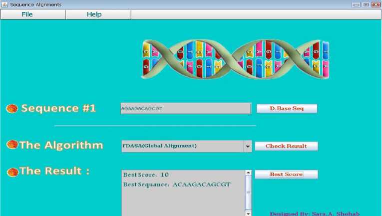
Fig. 7. The Best Score

• V.    Conclusions

In this paper, a modification of the global dynamic algorithm called EDAGSA is proposed. This modification depends on ignoring the unused data of the comparison matrix and evaluates the only three main diagonals of that matrix. The main idea of this modification is reducing the execution time, increasing the performance and decreasing the memory location that used to make the sequence comparisons. This algorithm is based on taking the advantage of dynamic algorithms that is getting the optimal solution for the sequences alignment. It also takes the advantage of the heuristic algorithm that it is decreasing the execution time for the sequence comparison. The complexity for both time and memory equals 3m+1 compared with m*n for the previous works. Also, for multi-sequences alignments the modified algorithm simply used the database to make comparison on it rather than files, thus we can do many comparisons in few milliseconds.

Acknowledgments

• [10]    Needleman, S. B. and C. D. Wunsch, A General Method Applicable to Search for Similarities in the Amino Acid Sequence of Two Proteins, Journal of Molecular Biology,48:443-453, 1970.

• [11]    Cormen, T. H., C. E. Leiserson, R. L. Rivest and C. Stein, Introduction to Algorithms, second edition, MIT Press, 2001.

• [12]    Smith, T. F. and M. S. Waterman, Identification of common molecular sub-sequences, Journal of Molecula Biology, 147:195-197, 1981.

• [13]    Bergroth, L., Hakonen, H. and Raita, T. "A Survey of Longest Common Subsequence Algorithms". SPIRE (IEEE Computer Society), 2000, 39–48.

Author’s Profiles

Arabi E. keshk received the B.Sc. in Electronic Engineering and M.Sc. in Computer Science and Engineering from MenoufiaUniversity, Faculty of Electronic Engineering in 1987 and 1995, respectively and received his PhD in Electronic Engineering from Osaka University, Japan in 2001. His research interest includes software testing, software engineering, distributed system, database, data mining, and bioinformatics.