Enhancement Processing Time and Accuracy Training via Significant Parameters in the Batch BP Algorithm

Published Online February 2020 in MECS

An artificial neural network (ANN) is a mathematical model inspired by biological node systems [1,2]. This is a description that offers great flexibility in modeling quantitative methods. The ANN has a strong ability to complete tasks many and is considered an active tool for training and classification[3-6]. An ANN provides a supervised learning algorithm which implements a nonlinear model within [0, 1] or [-1, 1], depending on the activation function [ 7, 8]. An ANN involves parallel processing, which consists of several parameters which need to be adjusted to minimize error training

Heuristic techniques are the most current methods for improving the training of the BBP algorithm. These methods include learning rate and momentum factor; these are significant parameters for adjusting the weights in training [ 9-10] . In general, the values of learning rate and momentum factor are fixed and are chosen from the interval [0, 1]. Manually set values for each training rate and momentum factor do not help the BBP algorithm escape from local minima or to meet the requirements of speeding up the training of the BBP algorithm.

Generally, there are two techniques for selecting the values for each learning rate and momentum factor. The first is set to be a small constant value from interval [ 0,1], the second the selected series value from[0,1], [11,12]. Therefore, one of the requirements for speeding up the BBP algorithm is adaptive learning rate and momentum factor together [13,14]. The learning rate should be sufficiently large to allow for escaping the local minimum to facilitate fast convergence to minimize error training. But the biggest value of the training rate leads to fast training with oscillation error training [15,16] .On the contrary, the small value of learning rate leads to reflex the weight that is lead to flat spot which makes BBP algorithm slow training [17,18]. The big values or small values are not suitable for smooth training. It is difficult to select the best or suitable values in training [19, 20].

The heuristic method is a current method for improving the BP algorithm, which covers two parameter training rate and momentum factor. The weaknesses, the values of training, rate and momentum are selected manual values. On the other hand, improves BP algorithm through creating dynamic training rate. But the weaknesses of these dynamic training depend on the initial value of training rate. Manually set values for learning rate and momentum factor do not help the BBP algorithm avoid local minima or meet the requirements of increasing training speed and difficult to choose a suitable value for learning rate and momentum factor. One way of avoiding localminima and speeding up the training of the BBP algorithm is to use a large value for training rate.

However, a small adjustment to the training weight slows the training of the BBP algorithm, while large adjustment to the weight results in unsmooth training. Most previous studies have tried to escape the local minimum through adaptive learning rates or momentum factors to improve the BBP algorithm. The persisting major problem, though, is the accumulation of weight in the BBP, which decreases accuracy and increases the time of training.

To fill the gap, we need to avoid the gross weight training, through creating dynamic parameter each learning rate and momentum factor with boundary to control the weight updated.

The remainder of this paper is organized as follows: Section II, literature review ; Section III, theoretically of training batch of back-Propagation algorithm; Section IV materials and method; Section V Created the dynamic learning rate and momentum factor, Section VI Experimental results; Section VII Discussion to validate the performance of improve algorithm; Section VIII Evaluation of the Performance of Improved Batch BP algorithm Section XI Conlusion.

• II.    Related Works

  Currently, works have been carried out, such as author, In [21] Improved back propagation Algorithm by adaptive the momentum factor by dynamic function. The dynamic function which proposed is depend on the two manual factors parameters. The learning rate selected by manual value to control the weight updated. Each factor and learning rate selected different value for each data set. To validate, this study through compares the performance of improved algorithm with BP algorithm.The proposed algorithm gave superior training algorithm than other with whole data set. In [22] improved the BP algorithm through two techniques, the training rate and momentum factor, values of training rate were fixed at different values. The idea of this study is to set the value of training, the rate to be large initially, and then to look at the value of error training after iteration. If the error (e) training is increased, the fit produced changes the value of training, rate multiplied by less than one and then recalculated in the original direction. If the iteration error can be reduced, this integration is effective. Therefore, by changing the training rate multiplied by a constant greater than one, the next iteration is calculated continuously. In[23] compared several techniques such as BP with momentum, BP with the adaptive learning rate, BP with adaptive learning rate and momentum, Polak-Ribikre CGA, Powell-Beale CGA, scaled CGA, resilient BP (RBP) conjugate gradient algorithm (CGA), and Fletcher-Reeves. The epochs of training are fixed with different values. The BP algorithm with adaptive learning rate and momentum gave superior accuracy training at 1000 epochs.

• III.    Theoretically of Training Batch of Back-Propagation Algorithm

In this section we will foucas on the theoretivall of BBP algorithm which cover the mathematical framework with significant parameters such as learning rate and momentum factor, and the gradient descent method. The BBP algorithm was designed to train models to achieve a balance between the actual data and the target correctly in the input patterns; this is done using the gradient descent method to minimize the error training of the BBP algorithm.

• A.    Mathematical Framework BBP Algorithm with γ and µ

The training BP algorithm is consist of three stages , namely ,forward propagation , in the feed forward phase , each input unit x receives an input signal x and broadcasts this signal to the next layer until the end layer in the system. The backward propagation this step is starting when the output of the last layer reach to end step then the start feedback. The end steep is update the weight, in the batch BP algorithm the weight adjustment stage for all layer adjusted simultaneously. The training of BP algorithm shown in the figure below

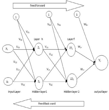
Fig.1. Batch BP algorithm stractur

The BP Algorithm with Training rate and Momentum term. The weight updates between the neuron k from output layer and neuron j from hidden layer as follows All steps training of the BP algorithm with training rate and momentum. Any neuron k from output layer and neuron j from hidden layer, the weight is adjusted between them as follows:

∆ w_jr ( t + 1) = w ( t ) - γ ^{∂ E} + µ ∆ w_jr ( t - 1)      (1)

w_jk ( t )

All steps training of the BP algorithm with training rate and momentum.

Forward Pass Phase: In this stage, the weight calculates layer by layer until reaching the end layer or output layer of the end layer under affected the activation function. Every variable f ′ ( x ) receives an input with initial weight and broadcasts to next the layer L ,..., L . The input signal L for each hidden unit is the sum of each input signal x . Each input layer as follows:

^L - inh

k

= u _{0 h} + ∑ u_ikx_i i = 1

Compute the output of first hidden layer of L

Lh = f (L-inh)(2)

Send the result to LL ( LL j = 1, 2,..., p ) and Calculate the input signal

LLj =v0h +∑vhjLh i=1

Calculate the output layer of second hidden LL

LLj = f (LL-inh)(4)

Send the output LL to input Y and then get the input layer of Y _{- inr}

k

Y-inh =w0h +∑LLJwjr(5)

i = 1

Compute theoutput layer of Y

^Yr ^{= f ( Y} - inr ⁾

Backward Pass Phase: when the weight reaches to the output of the last hidden layer to end step then the start all steps as follow

n er =∑(tr-Yr)(6)

r = 1

The local gradient of output layer Y at neuron r is defined by below equation

δr =erf(Y-inr), f'(Y-inr)=Y-inrf(1-Y-inr)(7)

Compute weight correction term (update later)

Δwjr = -γδrLLj + µ∆wjr(t-1)(8)

Calculate, bias correction term (update w г later

Δw0r = -γδ0r + µ∆w0r(t-1)(9)

Send δ to hidden layer , each hidden unite

LL_j , j = 1,..., p )

The single error or error back propagation from units in layer above to given as below

m

δ - inj = ∑ δ r W jr              (10)

r = 1

The local gradient of hidden layer LL at neuron j is defined by below equation

δj =-δ-inj f′(LL-inJ)(11)

Compute weight correction term (update v later)

∆vhj(t+1)=-γδjLh+µ∆whj(t-1)(12)

Calculate, bias correction (update v later)

∆vjr(t+1) = -γδj + µ∆v0r(t-1)(13)

Send δ to first layer h=1,…,q).

The single error or error backpropagation is given as below

b

δ - inh = ∑ δ j v hl                 (14)

j = 1

The local gradient of hidden layer L compute as follow ^'

h      - inh      - inh ,          - inr        - inr           - inr

Compute weight correction (update u later)

∆uih = -γδhxi + µ∆uih(t-1)(16)

Calculate bias weight corrective (used to update u later)

∆u0h = -γδh+ µ∆u0h(t-1)(17)

Update Weight Phase: the weight is update of the output layer j =(0,1,2,..., p;r = 1..., m) as follows wjr(t+1) =w(t) -γ∆wjr(t) + µ∆wjr(t-1)(18)

For Bias w0r(t+1) =w(t) -γδj + µ∆wjr(t-1)(19)

For each hidden layer  ( LL h = 0,..., q ; j = 1,... p )

vhj(t+1) =vhj(t) -γ∆whj(t) + µ∆whj(t-1)(20)

For Bias v0j(t+1)=v0j(t)-γ∆w0j(t)+µ∆w0j(t-1)(21)

For each hidden layer L ( i = 0,..., n ; h = 1,..., q )

uih(t+1) =uih(t) -γ∆uih(t) + µ∆uih(t-1)(22)

For Bias u0h(t+1) =u0h(t) -γ∆u0h(t) + µ∆u0h(t-1)(23)

The flowchart of the BP algorithm with trail value for each training rate and

• B.      Gradient Descent Backpropagation

Algorithm

The gradient descent method is one of the most popular methods used to  adjust the weight  for minimizing the training error in the BP algorithm [24, 25] Unfortunately, the gradient descent method is not guaranteed to find the global error [26, 27] .It may, therefore, result in leading to a local minimum, as the gradient descent method is not powerful enough to adjust for the weight, apart from limited changes [28] .The batch gradient descent method computes gradients using pattern training and updates the weight in the final stages of training [29]. This method focuses on modifying one parameter or more than one as adaptive of activation function or modifying the gain. The value of the gain is seen in the effect of the behavior of the convergence algorithm [30]. The author [31] proposed a new algorithm through the modified gain in the activation function. The proposed algorithm gives superior training compared with the BBP an algorithm.

Gradient descent ∆ E taken partial of the differentiate of error with respect the weight w in each layer. ANN which is consist one input, one hidden layer and one output also focus for one neuron as k from output layer and one neuron j from hidden, as follows

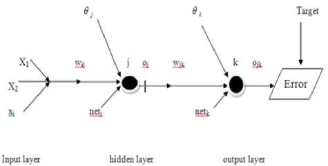
Fig.2. Gradient Descent for one Hidden Layer

1 ^k

Let the error training is given by E = ∑ ( t - o )² , 2 k = 1

activation function of training is sigmoid function

f ( x ) =             . When the gain equals is one. The

• 1    + Exp ( - x )

weight update between the neuron K , from output and neuron j from hidden layer as follow

A w k ( new ) = A w k ( old ) - / А w k + ^A v hj (t - 1)    (24)	d E =   8 E   8 net k d oj   d netk   8 oj
The gradient between neuron K from output layer and neuron j from hidden layer	Insert equation (35) into equation (34) it becomes as below
d E     8 E   8 ojk   8 netk A w ,k =      =        ---- (25) d W jk    d o k 8 net k  wjk	8 E     8 E   8 netk   8 o -----------—           (36) d net,.    8 net,    8 o,    8 net, j   kj   j
d E   1 d ,        2 a = i a   ( tk  ok ) 8 o k   2 8 o k	A     8E     8 E   8 netk   8 o j   d net j A w =--------------- (37) 5 w„    5 net,    d o,    8 net,   8 w„ ij               k           j               j           ij
I E" = - ( t k - o k )              (26) d o k	8 E _ 8E   8 ok d netk    d ok d netk
d o jk ;     8       1 d netk    8 netk 1 + e - x	8E — = - ( tt - o k ) o k (1 - o k )          (38) d netk
8 oik -=- = ok (1 - ok )              (27) d netk	Put 5 k = ( t t - o k ) o k (1 - o k ) then get
■'   •  = x,                         (28) w jk	= 5 k                   (39) d netk
Insert equation 25, 26, 27 into equation (25) it becomes as follow	dnetk    8  .j        ... —- = —(/ o,w„ + 9, ) 8 o j     8 o j ^ j ij   j
A w jk = - ( t k - o k ) o k (1 - o k ) x j           (29)	d netk k = W y                   (40) 8oj
Insert equation (29) into equation (24) to get a new equation for update the weight as below	.5 o j =_8 L *„ 1
A w jk ( new ) = A w jk ( old ) - / ( t , - o k ) o k (1 - o k ) x j  (30)	d nety    d nety ( 1 + e j )
Put the 5. = ( tk - ok ) ok (1 - Ok ) then get the equation	6 o, -=- = f '( netj ) = Gy (1 - Gy )           (41) 6 netj
A w k ( new ) = w jk ( old ) + n§ k x j         (31)	8 net      8 ( к          A
For calculate the local gradient between neuron j from hidden layer and neuron i from input layer. In this case the weight update as follow	------=---- / XiWii + 9, 8 W ,j    8 W j ( k = 1          J 8 net, --x- = x              (42)
A W j ( t + 1) = W j ( t ) - yA W j ( t )          (32)	d Wj
The gradient between neuron j from hidden layer and neuron i from input layer given as follow	Insert equation (26, 27, 28) into equation (25) it becomes as below
BE    8E 8 net, — = — ---(33) 5 W  5 nety d Wy	A W =     = - ^ ( t t - o k o (1 - o k > w yo^ (1 - o j > x d W lj      k = 1
5=dE .j^         (34) 8 nety    8 oj 8 nety	From equation (29) replace ( tt - ok ) ok (1 - ok ) by 5

∂ E

∆w = ij   ∂Wij

-

∑ δ _kw_ijo_i (1 - o_j ) x_i k = 1

Put δ j = ∑ ^{j = i} δ k w ij o i (1 - o j ) in (42) to get j = 1

∂ E

∆w== ji    ∂W

Insert (43) into equation (32), then the weight update between neuron j from hidden layer and neuron i from input layer as below

∆W (new) = w (old) +γδ x(45)

• IV.    Materials and Method

This kind of this research belongs to the heuristic method. This method includes the learning rate and momentum factor. To investigate the aims of this study there are many steps as follows:

• A.    Data set

The data set is very important for verification of improved DBBPLM algorithm. In this study, all data are taken from UCI Machine Learning Repository through the link All real data set to change to become nomination data set between [0,1] and divided into two set training set and testing set.

• B.    Neural Network Model

We propose an ANN model, which is a three-layer neural network that has an input layer, hidden layer, and output layer. The input layer is considered to be { x ₁, x ₂, , x }, which represents the nodes; the nodes depend on the types or attributes of the data. The hidden layer is made of two layers with four nodes. The output layer Y is made of one layer with one neuron. Three basis, two of them are used in the hidden layers and one in the output layer. Finally, the sigmoid function is employed as an activation function

• V.    Created the Dynamic the Prameters Learning Rate and Momentum Factor

The weight update between neuron k from the output layer and neuron j from the hidden layer ( w ) in equqtion (1) which recorded as above.

To enhance the BBP algorithm, which is given by the Equation above (1) to avoid the local minima and to avoid saturation training. The learning rate should be sufficiently large to allow escape from the local minimum and to facilitate fast convergence to minimize error training . However, the value of the learning rate which is too large leads to fast training with an oscillation in error training. To ensure a stable learning BP algorithm, the learning rate must be small. Depend on above, we will create the dynamic training rate with boundary to keep the weight as moderate as follows:

sec h ( sh (1 - sh ) γ _dmic = + exp( sh . e ) (46)

Where the sech θ is Hyperbolic functions, θ is angle, and the sech θ = 2/( e ^θ + e ^{- θ} ) . The sh(1-sh) is slop the first derivative of the activation function of the out put of second hidden layer and (e) is the error training. We can see the value of ( sh ) is located between 0 and 1, the value of ( sh ) is a boundary. In the same way, the training error ( e ) is boundary value 0 ≤ e≤ 1. Each sh and e boundary function, that is lead to sh×e is boundary function, 0 ≤sh×e≤1. Depend on the above we can find the 1≤ ≤2.78 . the dynamic γ is boundary funcation.

The second significant parameter is momentum. To get smooth training and avoid inflation in the gross weight of the added values for momentum factor, the fitting producer through creating dynamic momentum factor and implicate the Depend above we can create the dynamic momentum factor µ as follow sech(sh(1 - sh)

+ exp( sh . e )

We Insert the equation (46) and (47) into equation (1), then the weight is updated between any layer as below sech(sh(1-sh)              ∂E wjk(t+1)=wjk(t)-[                 + exp(sh.e)]

2                        w_jk ( t )

+

sec h ( sh (1 - sh )

+ exp( sh . e )

∆ w_jk ( t - 1)

For the equation (48) the dynamic algorithm will be updated the weight under affected the dynamic learning rate and dynamic momentum factor.

• VI.    Experimental Results

The accuracy of training is calculated as follows [32,33]

1-absolut(T -O )

Accuracy (%) =         i i ∗ 100 where UP and LW are the upper bound and lower bound of the activation function.

• A.    Experimental Results for the DBBPLM Algorithm Using the XOR Problem

Ten experiments were carried out using Matlab, and the average (AV) was taken for several criteria used for measurement of the training performance. Ten experimental has been done for DBBPLM with XOR and then taken the average and S.D.The average and S.D of experimental results are tabulated in Table 1.

Table 1. Average the Performance of DBBPLM algorithm with XOR

	Time-sec	Epoch	MSE	Accuracy
Average	2.2463	1681	9.998E-05	0.9859
S.D	0.36127166	0	0	2.22E-16

From Table 1., the formulas proposed in equations (46 and 47) help the back-propagation algorithm to enhance the performance of the training. Whereas the average time training is t = 2.2463 seconds and the epoch is 1681 epoch. The smallest value of standard deviation S.D indicates the scatter of time or error training is very close for every experiment, whereas the S.D = 0.36127166 second. The accuracy rate is 0.9859.

• B.    Experiment result of the BBP algorithm with XORProblem

For the dynamic DBBPLM algorithm we run the dynamic algorithm 10 time with XOR problem and then take the averge for time , epoch and accuracy rate as follow

Table 2. Performance of BBP algorithm with XOR

Value of		times	MSE	Epoch
γ	µ
0.1	0.004	52.4760	9.999e-05	67490
0.0001	0.0001	6530	0.5011	194345
0.004	0.95	5670	1.635e-04	153329
0.1	0.1	55.9070	9.999e-05	76190
0.2	0.2	31.0090	9.997e-05	37839
Average		2467.8784	0.1003127	105838.6
S.D		2978.0706	0.2003937	58416.301

From Table 2., the range of the training time is 31.0090.0090≤ t≤ 6530 seconds. We consider the value 31.0090second is as minimum training time and the value6530 second is as maximum training time. The best performance of the BP algorithm is achieved at γ = 0.2 and at µ =0.2 whereas the training time is 21.0090 seconds, the worst performance of the BP algorithm is achieved at γ = 0.0001 and µ =0.0001 for first, whereas the training time is 65300 second.

• C.    Experiments result of the DBBPLM algorithm with Balance- Train set

We implement the DBBPLM algorithm ten time with the balance data training set. and then the average was taken for several criteria. The experiment's result is tabulated in the Table 3.

Table 3. Average the Performance of DBBPLM algorithm with Iris- Train set

	Time-sec	Epoch	MSE	Accuracy
Average	3.3663	61	9.887E-05	0.992
S.D	1.55506733	13.169662	9.139E-07	0.0016697

From Table 3., the dynamic approach for training rate and momentum term reduce the time required for training and enhance the convergence of the time training. The average training time is 3.3663 seconds at an average epoch is 61 epochs. The average accuracy training is 0.992

• D.    Experiments of the BBP Algorithm with BalanceTrain set

We tested the BBP algorithm with several optimum values. The experiments result recorded as table V with iris –training set

Table 4. Performance of BBP bbp algorithm with Iris- Train set

Value of		times	MSE	Epoch
γ	µ
0.1	0.004	67.5020	9.7199e-05	323
0.01	0.25	61.5210	9.8827e-05	1129
0.004	0.95	220.0530	9.9736e-05	4361
0.005	0.09	153.8200	9.9950e-05	2993
0.005	0.001	179.8890	9.9960e-05	3535
Average		129.157	9.913E-05	2468.2
S.D		71.7656181	1.053E-06	1509.4044

From Table 4., the best performance of the BP algorithm was at γ = 0.01 and µ =0.25 whereas the time training is 61.5210 ≈ 52 second while the best performance of the BP algorithm is achieved at γ = 0.004 and µ =0.95 whereas the time training is 220.0530 ≈ 220 seconds. In addition, the range of the average training time is 61.5210≤ t ≤ 220.0530seconds.

• E.    Experiments result of the DBBPLM Algorithm with Balance- Testing set

Ten experiments has been done with balance testing and then taken the average of several criteria. The experiment result is tabulated in the Table 5.

Table 5. Performance of DBBPLM with Iris- Testing set

	Time-sec	Epoch	MSE	Accuracy
Average	3.6801	88	9.821E-05	0.9906
S.D	0.98730577	20.813697	1.143E-06	0.0019355

From Table 5., the average training time is 3.6801 seconds at an average epoch is 88 epoch. The average S.D of time is 0.98730577. The accuracy rate is very highest about 0.9887.

• F.    Experiments result of the BBP Algorithm with Balance- Testing set

We tested the BBP algorithm with several optimum values. The experiments result recorded in the Table 6., with iris –testing set

From Table 6., the best performance of the BP algorithm was at γ = 0.1 and µ = 0.1, whereas the time training is 79.9910 ≈ 80 seconds, while the worst performance of the BBP algorithm is achieved at γ =0.0001 and µ =0.0001 whereas the time training is 5600 second. The range of the average training time is 79.9910≤ t ≤ 5600 seconds. The average S.D of time is greater than one.

Table 6. Performance of BBP Algorithms with Iris- Testing set

Value of		times	MSE	Epoch
γ	µ
0.1	0.004	79.9910	5.5408e-05	2867
0.0001	0.0001	5600	0.2049	96800
0.005	0.09	4868	0.8193	7352
0.005	0.001	1.422e+3	5.0238e-05	39854
0.01	0.25	591.4530	5.0937e-05	14140
0.1	0.1	70.0050	5.6064e-05	1840
Average		2105.2415	0.1707354	27142.167
S.D		2267.46456	0.2995366	33674.904

• G.    Experiments result of the DBBPLM Algorithm with Iris.- Train set

Table 7. Average the Performance of DBBPLM Algorithm with Balance - Train set

	Time-sec	Epoch	MSE	Accuracy
Average	9.9023	77	2.9658e-04	100
S.D	0.52140945	0	0	0

From Table 7., the experiments result indicates the dynamic learning rate and momentum factor helps the BBP algorithm for reducing the time training. The average time is 9.9023 ≈ 10 seconds with 77 epoch. The average S.D of time is 0.52140945. .

• H.    Experiments result of the BP Algorithm with Balance - Train set

We test the manual algorithm at several values for each learning rate and momentum factor. The result are recoded in the Table 8.

Table 8. Performance of DBBPLM Algorithm with Balance - Train set

Value of		times	MSE	Epoch
γ	µ
0.1	0.004	105.5750	9.996e-05	6882
0.004	0.95	96.5370	1.0000e-04	6176
0.005	0.09	1.85e+3	9.99e-05	124715
0.005	0.001	4963	1.185e-04	117460
0.1	0.1	93.0560	9.98e-05	6289
0.2	0.2	76.7300	9.91e-05	9554
Average		1197.483	0.0001029	45179.333
S.D		1197.483	0.0001029	45179.333

From Table 8., the range of the training time is 76.7300≤ t ≤ 105.5750 seconds, the range of training time is very widely.

• I.    Experiments result of the DBBPLM Algorithm with iris.- Testing set

Table 9. Average the Performance of DBBPLM Algorithm with Balance - Testing set

	Time-sec	Epoch	Accuracy
Average	6.482	76	0.9860
S.D	0.3571277	0	0

From Table 9., the average time is 6.482 6 seconds with 76 epochs. The accuracy rate is 0.9860, the accuracy rate is the nearest one

• J.    Experiments result of the manually BBP Algorithm with Iris.- Testing set

We test the manual algorithm at several optimum values for each learning rate and momentum factor . The result are recoded in the Table 10.

Table 10. Performance of BBP Algorithm with Balance - Testing set

Value of		Time-S	MSE	Epoch
γ	µ
0.1	0.004	81.9550	2.772e-4	11490
.0001	0.0001	4976	0.0077	369071
0.004	0.95	3693	0.0077	152912
0.005	0.09	3546	5.35e-04	129706
0.005	0.001	1.97e+03	2.68e-04	273293
0.1	0.1	94.9780	2.76e-04	9833
0.2	0.2	75.6650	2.979e-04	5204
Average		2062.514	0.0024363	135929
S.D		1893.50603	0.0033302	132031

From Table 10., the range of the average training time is in the interval 75.6650 ≤ t ≤ 4976 seconds this means the range of time training is wide. The best performance of the BP algorithm is achieved at у = 0.2 and Ц =0.2 the worst performance of the BP algorithm is achieved at / = 0.0001 and µ =0.0001. The BBP algorithm suffers the highest saturation at γ = 0.0001 and µ =0.0001.

• VII.    Discussion to Validate the Performance of Improved Algorithm

To validate the efficiency of the improved algorithm, through comparing the performance of the DBBPML algorithm with the performance of the batch BP algorithm based on certain criteria[34, 35].We calculate the speed up training using the following formula [36].

Proccessing Time

Execution time of BBP algorithm

Execution time of DBBPLM algorithm

In this part we will compare the performance for each DBBPLM dynamic algorithm which listed in the from Table.1, 3,5,7,9 with the performance of manually algorithm wich listed in the Tables 2,4,6,8,10. The comparission result are tabulated in Table 11.

Table 11. Processing Time Improved the DBBPLM Algorithm versus BP with first structure

	Dynamic (DBBPLM)algorithm		A manually BBP algorithm
	AV Time	AV Epoch	AV Time	AV Epoch	Processing Time Improved
XOR	2.2463	1681	2467.8784	105839	1098.641499
Balance Training	9.9023	77	1197.483	45179	120.929784
Balance Testing	6.482	76	2062.514	135930	318.1909904
Iris Training Iris	3.3663	61	129.157	2468	38.367644
Testing	3.6801	88	2105.2415	27142	572.0609494

From Table 11., it is evident that the dynamic algorithm provides superior performance over the Manually algorithm for all datasets. The range of the training time of the Dynamic algorithm is 2.2463 ≤ t ≤ 9.9023 s; this is a narrow interval, meaning that the dynamic parameters which created help the algorithm to reaches the global minimum in a short time and with few epochs. The range of training times of the BBP algorithm is 129.157 ≤ t ≤ 2105 s; this is a wide interval, meaning that the BBP algorithm has a long training time and a high level of training saturation. The dynamic algorithm is 2360.166 ≈ 2360 times faster than the BBP algorithm at its maximum.

Easily we can see in the end Column in the table above, dynamic algorithm which created in this paper gave faster training than manual algorithm. For example the dynamic algorithm is 1098.641499se 1099 time faster than manual algorithm at its maximum time training. Also dynamic algorithm which created in this paper gave faster training than manually algorithm. For example the dynamic algorithm is 38.367644se 38 time faster than manual algorithm at its minimum time training

From Figure 3 Obviously, we can see the dynamic algorithm taken a short time to reach the glob minimum, for all data set while the Manual algorithm takes a long time to reach a global minimum. The dynamic algorithm created in this study is able to escape the local minimum and remove the saturation training.

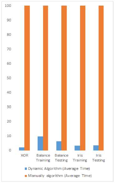
Fig.3. The performance of Dynamic algorithm versus Manually algorithm for time

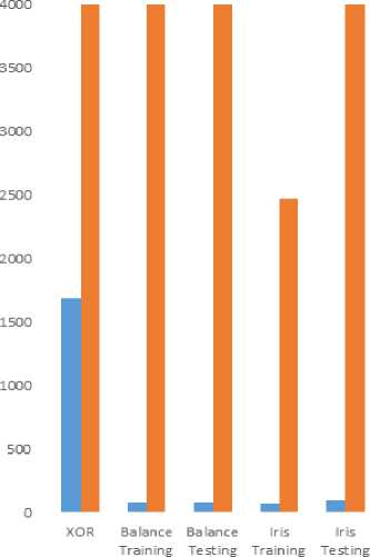
■ Dynamic Algorithm (Average Epoch)

■ Manually algorithm (Average Epoch)

Fig.4. The performance of Dynamic algorithm versus Manually algorithm for epoch

From Figure 4 it is evident that the dynamic algorithm which created in this study provides superior performance over the Manually algorithm for all datasets. The dynamic algorithm taken few epochs to reach to the global minimum while the Manual algorithm takes a big value of epochs to reach the global minimum.

• VIII.    Evaluation of the Performance of Improved Batch BP Algorithm

  To evaluated the performances of the improved batch BP algorithm for speeding up training the performances of the improved batch BP algorithm are compared to previous research works such, Hameed et al (2016) and Azami, (2015), the stop training for both study determined by number of iteration, the number iteration set by 2000 iteration and 1000 iteration respectively. For the purpose of the comparison between the results of this study and the previous works, the fit is re-run again with different stop training values according to previous work. The performance of the improved algorithm which proposed in this study give superior performance than exists works.

• IX.    Conclusion

We have introduced the dynamic DBBPLM algorithm, which trains by creating a dynamic function for each the learning rate and momentum factor. Sevral dataset were used, all data are taken from the UCI Machine Learning Repository through the following link: All datasets should be changed to become normalized in the interval [0, 1]. The dataset was divided into two sets, a training set and a testing set for validating the performance of the contribution. This function influences for the weight. Of the DBBPLM algorithm were carried out on Matlab 2012a with same goal error or limited error training. One of the main advantages of the dynamic training and dynamic momentum factor are reduces the training time, the training error, number of epochs and enhancement the accuracy of the training. The performance of dynamic DBBPLM algorithm which presented in this study gave superior performance compared with exists work.