Evaluation of Interest Point Detectors in Presence of Noise

Автор: Adrian Ziomek, Mariusz Oszust

Журнал: International Journal of Intelligent Systems and Applications(IJISA) @ijisa

Статья в выпуске: 3 vol.8, 2016 года.

Бесплатный доступ

Detection of repeatable keypoints is often one of the first steps leading to obtain a solution able to recognise objects on images. Such objects are characterised by content of image patches indicated by keypoints. A given image patch is worth being described and processed in further steps, if the interest point inside of it can be found despite different image transformations or distortions. Therefore, it is important to compare keypoint detection techniques using image datasets that contain transformed or noisy images. Since most of detector evaluations rely on small datasets or are focused on a specific application of compared techniques, in this paper two large datasets which cover typical transformations, as well as challenging distortions that can occur while image processing, are used. The first dataset contains 200,000 transformed images, and it has been prepared for the purpose of this study. The second dataset, TID2013, is widely used for perceptual image quality assessment; it contains 3,000 images with 24 distortions. Finally, interest point detectors are evaluated on four datasets, and repeatability score and time of detection are used as measures of their performance.

Еще

Keypoint, interest point detectors, distortions, noise, repeatability, evaluation, pattern recognition

Короткий адрес: https://sciup.org/15010802

IDR: 15010802

Текст научной статьи Evaluation of Interest Point Detectors in Presence of Noise

Published Online March 2016 in MECS

Interest point detectors and descriptors, which characterise the detected image region, are fundamental concepts in many fields of computer vision and robotics, widely used in vision-based object recognition, tracking, or localisation. They have been the target of intense research activity in the past few years.

An interest point (a keypoint, or a corner) is a spatial location in the image associated with content which can be useful for further processing [1-2]. In general, the importance of information carried by the local image content is application dependent, and therefore many different keypoint detection schemes have been proposed. Furthermore, there are different approaches trying to define what local neighbourhood should contain in order to be classified as the interest point. For example, often a brightness change or some texture is taken into consideration.

The most desirable property of a detector is its ability to find repeatable keypoints, and repeatability is regarded as the one of the most important property of keypoint detection schemes. This means that a given image patch is worth being processed if the interest point inside of it can be found despite different image transformations, distortions or in presence of noise.

The remaining part of the paper is organised as follows. Section II describes related works on evaluation of keypoint detectors. Section III gives background information concerning detectors. The evaluation framework is presented in Section IV, and performed experiments are in Section V. Finally, conclusions and future works are presented in Section VI.

II. Related Works

Many comparative tests have been conducted in order to evaluate state-of-the-art keypoint detection schemes [1-10]. Among measures of detectors’ performance one can find time of detection, repeatability, the number of correspondences, matching score, or the number correct matches. The first two measures evaluate detectors, while other are more focused on descriptors.

Many evaluations present results for combination of detectors with descriptors, however they admit that such combinations are often application dependent. For example, authors in [5] tested suitability of algorithms for fall detection systems, where orientation invariance is taken into account or, as in [6], compared two keypoint detectors and descriptors using natural outdoor environment images. There are also approaches testing suitability of keypoint detection techniques for 3D applications [11-13].

Comparison of interest point detection approaches often rely on small datasets with several image transformations. Therefore, this paper presents a study in which apart from two typically used image datasets,

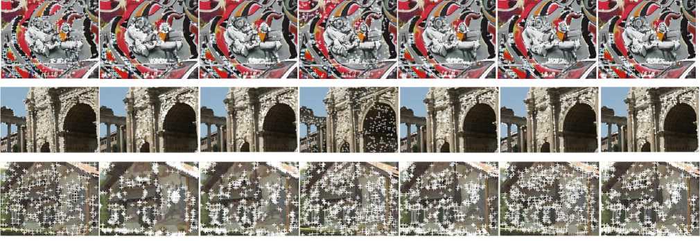
Fig.1. Detection results for evaluated detectors: FAST, KitRos, Median, SIFT, KLT, SURF, and Harris (from left to right). Interest points are denoted with white crosses.

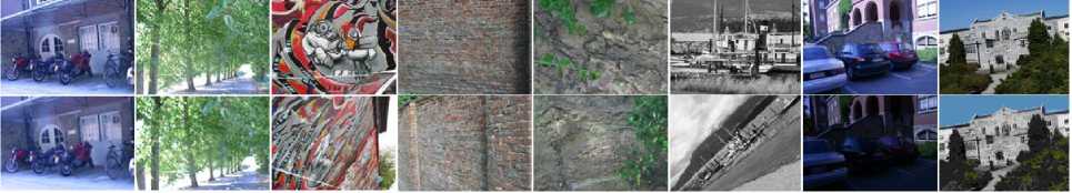
Fig.2. Reference images and their exemplary transformed images from Mikolajczyk and Schmid dataset [2]. The following image sequences are presented: Bikes, Trees, Graffiti, Wall, Bark, Boat, Leuven, UBC (from left to right; transformed images are in the second row).

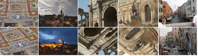
Fig.3. Reference images and their exemplary transformed images form Heinly et al. dataset [3]. The following image sequences are presented: Ceiling, Day and night, Rome, Semper, Venice (from left to right; transformed images are in the second row).

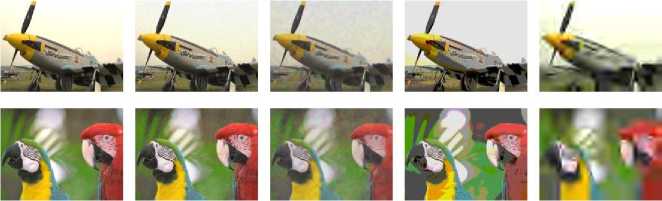
Fig.4. Two reference images from TID2013 dataset [24] (in the first column) and their distorted equivalents.

Fig.5. One reference image from [25] and its transformations.

descriptors are evaluated on a large dataset that has been prepared for the purpose of this study, and a dataset used in the field of image quality assessment. The first dataset contains simple image transformations, such as rotation, scaling or Gaussian blur, but the large number of testing images allows drawing conclusions on the general performance of a given detector. The second dataset contains 24 different image distortions and their levels. It supports examination of compared detectors in presence of noise. In this work, the visible lack of such investigation in the literature is addressed. Finally, seven of detection time and repeatability score. widely used interest point detectors are evaluated in terms

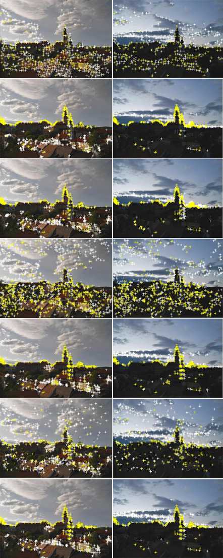
Fig.6. Detection results for evaluated detectors on exemplary original image (left column) and its equivalent (right column): FAST, KitRos, Median, SIFT, KLT, SURF, and Harris (from top to bottom). Interest points that are present in both images are denoted with yellow crosses.

III. Interest Point Detectors

The representative interest point detection techniques are described in subsections below. Exemplary results of their usage can be seen on Fig.1.

A. Harris Detector

In the one of the first attempts to the design of a keypoint detector, Moravec [14] proposed to consider an interest point, or a corner, to be a point that is characterised with a low self-similarity. The similarity is computed using sum of squared differences between pixels which belong to the considered image patch and other image patches in its neighbourhood. Harris and

Stevens in [15] used the differential of the corner score, and in order to address isotropy issue of Moravec’s approach, the score was computed taking into account direction of the shift. Authors pointed out that the corner is likely to be found if the first two eigenvalues of the autocorrelation matrix, characterising a given image patch, have large positive values. Instead of calculating time consuming eigenvalues, authors used the determinant and the trace of the matrix.

B. KLT Detector

KLT (Kanade–Lucas–Tomasi) detector [16, 17] is similar to the Harris method. The main difference is change in the calculation of the corner response. In KLT , two gradient matrices representing two image patches are examined in order to determine minimal eigenvalue. This technique is often used for tracking, where the difference between compared image patches is minimised.

C. KitRos Detector

In an approach proposed by Kitchen and Rosenfeld [18], the corner measure is calculated as a product of a local gradient magnitude and a rate of change of gradient direction.

D. Median Detector

This keypoint detector is based on median filter. Median filtration assigns each pixel of the image a median value calculated taking into account its neighbourhood. Median-based filter detector works by subtracting the filtered image from the original one.

E. FAST

FAST (Features from Accelerated Segment Test) detector [19] uses circle of 16 pixels to classify points as corners. Points around the pixel are labelled from integer number 1 to 16 clockwise. If n adjacent pixels are darker or brighter than the centre pixel plus a constant, such location is considered an interest point. To make this computation faster, only first 1, 5, 9, and 13 pixels are checked.

F. SIFT

SIFT (Scale Invariant Feature Transform) is a method proposed by Lowe in [20]. The algorithm is both keypoint detector and descriptor. The first step in keypoint detection is to create scale space representation of the image by repeatedly convolving the image with a Gaussian filter. Then, Difference of Gaussian (DoG) and interpolation over the scale-space are used in order to find the locations of stable scale-invariant keypoints. Orientation invariance is achieved by assigning to each point its orientation. Keypoint descriptor is formed as a normalised vector of 128 elements obtained from gradient orientations and magnitudes.

G. SURF

SURF (Speeded Up Robust Features) [21] approach is inspired by SIFT. Like SIFT, it is also both interest point detector and descriptor, able to find features invariant to scale and rotation. For detecting keypoints, SURF uses an integer approximation of the determinant of Hessian blob detector (DoH), which can be computed with three integer operations using a precomputed integral image. Sum of Haar wavelet response around the keypoint is used to create the descriptor. SURF runs faster than SIFT due to approximations and usage of integral image technique.

IV. Evaluation Framework

For evaluation of compared interest point detectors, we used two measures of their quality, i.e., repeatability and time of detection. In some works, (e.g., in [3, 7]), detectors are also coupled with descriptors and keypoint matching is performed or other related task, such as image recognition. The results of the latter tests are mostly application dependent and different detectors are recommended as being the best. Therefore, in this work we will focus on repeatability, since it is highly demanded, and time of detection, which often determines the practical usage of the detector.

A. Repeatability

A keypoint is said to be repeatable if the distance d between its location and the location of the nearest keypoint (in pixels) that was found after introducing a distortion to the image is less than ε [11, 12, 19]. Benchmark datasets often provide homography between images used in order to determine expected keypoint location. Repeatability score is calculated as the percentage of points simultaneously present in two images, taking into account ε .

B. Detection Time

Detection time, t_d , can be considered as the one of the most practical evaluation measures, since it may influence the choice of the detector for real-time applications.

C. Datasets

We used four datasets for the evaluation of compared approaches. Mikolajczyk and Schmidt [2] and Heinly et al. [3] datasets are typically used for evaluation of interest point detectors and descriptors. The first one contains eight images with gradually introduced following image transformations (six distorted images for each reference image): blur, viewpoint, zooming with rotation, brightness change and JPEG compression. Reference images and exemplary distortions from this dataset can be seen on Fig 2. Heinly et al. dataset contains five reference images and from six to nine their corresponding transformed images. In this dataset, only rotation, illumination and scale changes are taken into account. Reference images along with some of their distorted images are presented on Fig. 3.

Since these popular datasets allow evaluating only a limited number of distortions and the number of distorted images is small, we decided to use a dataset that contains distorted images for the purpose of perceptual quality assessment [22, 23]. Tampere Image Database 2013 [24] (TID2013) contains 25 reference images, 24 types of distortions and five levels of distortions (3,000 images in total). The dataset is prepared for evaluation of image visual quality assessment metrics; however we used it to evaluate keypoint detectors in presence of most popular distortions. Two images and their exemplary distorted equivalents are shown on Fig. 4. Furthermore, in order to provide evaluation using distortions that are not present in TID2013, i.e., scaling and rotation of the image, we have created our own large scale dataset on the basis of MIRFLICKR25000 dataset [25]. The original dataset contains 25,000 Flickr images, we have altered them introducing rotation (45º and 90º) and scale (x, y ={0.6, 0.6}, x, y = {0.3, 0.3}, x, y = {1, 0.6}, x, y = {0.6, 1}). To the resulting dataset we also added images distorted with Gaussian blur (σ = 2, σ = 4). Similar transformations can be found in [10]. Finally, 200,000 images have been obtained. One reference image and its transformed equivalents are presented on Fig. 5.

V. Experiments

Experiments were performed on i5-4300U CPU, using JAVA implementations of keypoint detectors that are available in BoofCV library [26]. The choice of this computer vision library was motivated by the quality of obtained results reported in [26] and lack of comparison of interest point detection techniques implemented in JAVA. All compared methods were run with their default parameters. Repeatability score was calculated with threshold ε = 5 pixels. Since the score favours approaches that detect more keypoints, we used 500 keypoints with the strongest response in experiments. If the number of detected keypoints was smaller for one technique, the same number of keypoints for other techniques was used.

The detailed presentation of the results for every pair of compared images is not possible for larger datasets; therefore our discussion will be supported with mean values of obtained repeatability scores on TID2013 and modified MIRFLICKR25K datasets. The comparison of detectors for smaller datasets is presented using mean values as for large datasets but also on a level of results obtained while matching reference image with its transformed images. For the first two datasets, testing images are numbered starting from two.

Table 1 contains repeatability scores for Mikolajczyk and Schmidt dataset. Here, the best result is written in boldface. Harris detector together with KLT outperformed other detectors on this dataset. It is worth noting that the dataset contains only several types of transformations. As one can see, for image sequences with blur and light changes SURF was better than other counterparts. However, this advantage was only clear for Trees sequence. Similar results have been obtained on Heinly et al. dataset; they are presented in Table 2. This dataset contains mostly sequences of images with rotation, and in their case Harris and KLT detectors were superior to other techniques. It happened also for Day and night sequence, where illumination changes are present (see Fig. 6).

Table 1. Repeatability Scores (in %) Obtained on Mikolajczyk and Schmidt Dataset. The Best Approach for Each Transformation is Written in Boldface

Transformation: scaling+rotation, image sequence: Bark

Image no	SURF	KLT	SIFT	KitRos	Median	FAST	Harris
2.0	44.8	37.4	36.6	27.4	31.2	28.8	39.2
3.0	22.6	17.0	9.6	19.0	17.6	16.0	22.0
4.0	25.2	48.2	14.4	38.2	41.2	22.0	47.6
5.0	24.0	45.0	18.4	38.6	48.8	25.2	51.0
6.0	16.6	33.6	11.8	34.0	39.0	18.0	41.8
Mean	26.6	36.2	18.2	31.4	35.6	22.0	40.3
	Transformation: blur, image sequence: Bikes
Im. no	SURF	KLT	SIFT	KitRos	Median	FAST	Harris
2.0	77.6	75.2	60.0	64.8	63.4	54.6	78.2
3.0	77.2	72.2	54.8	59.8	54.8	54.2	74.2
4.0	65.2	63.0	40.8	53.4	47.8	44.8	66.4
5.0	60.8	61.0	33.8	48.8	44.0	35.7	61.0
6.0	31.2	43.4	19.4	36.2	36.0	30.6	46.0
Mean	62.4	63.0	41.8	52.6	49.2	44.0	65.2
Transformation: scaling+rotation, image sequence: Boat
Im. no	SURF	KLT	SIFT	KitRos	Median	FAST	Harris
2.0	70.2	81.6	47.6	65.0	69.4	55.2	83.8
3.0	62.8	81.2	28.4	59.0	70.6	45.2	84.8
4.0	51.8	79.8	15.6	70.4	70.2	32.8	82.0
5.0	46.2	85.6	14.0	70.8	72.2	29.8	85.4
6.0	39.8	68.8	14.6	54.2	56.0	20.4	67.8
Mean	54.2	79.4	24.0	63.9	67.7	36.7	80.8
	Transformation: viewpoint, image sequence: Graffiti
Im. no	SURF	KLT	SIFT	KitRos	Median	FAST	Harris
2.0	24.8	18.4	17.4	15.4	18.0	14.6	19.4
3.0	16.0	15.4	14.4	15.0	16.6	13.0	18.4
4.0	11.4	13.4	13.6	11.8	11.6	11.0	15.4
5.0	10.8	10.0	9.4	8.8	9.8	11.8	12.0
6.0	11.2	6.0	11.4	7.6	6.2	8.8	6.6
Mean	14.8	12.6	13.2	11.7	12.4	11.8	14.4
	Transformation: light, image sequence: Leuven
Im. no	SURF	KLT	SIFT	KitRos	Median	FAST	Harris
2.0	24.8	20.4	11.6	20.2	19.0	14.2	20.6
3.0	23.0	19.0	13.0	20.8	17.4	11.6	19.0
4.0	22.6	18.4	15.2	19.0	18.6	14.6	18.4
5.0	0.0	0.0	0.0	0.0	0.2	0.0	0.0
6.0	18.0	17.0	14.6	15.8	16.6	16.7	18.4
Mean	17.7	15.0	10.9	15.2	14.4	11.4	15.3
	Transformation: blur, image sequence:					Trees
Im. no	SURF	KLT	SIFT	KitRos	Median	FAST	Harris
2.0	51.0	46.4	38.8	31.8	39.6	35.4	54.8
3.0	41.8	39.6	25.2	22.2	27.4	23.4	38.8
4.0	33.4	30.2	25.2	18.4	19.0	21.4	32.0
5.0	42.0	27.2	22.8	15.0	13.0	18.4	23.6
6.0	34.6	23.2	12.8	12.4	9.4	12.2	20.2
Mean	40.6	33.3	25.0	20.0	21.7	22.2	33.9
Transformation: JPEG compression,					image sequence: UBC
Im. no	SURF	KLT	SIFT	KitRos	Median	FAST	Harris
2.0	93.4	92.8	76.0	76.2	86.6	70.2	97.4
3.0	88.8	92.0	56.6	69.8	78.0	62.6	93.8
4.0	82.4	89.4	56.0	66.0	71.2	57.4	91.2
5.0	74.4	85.4	39.6	59.4	65.0	43.6	83.4
6.0	67.4	80.8	31.0	58.0	57.8	40.3	78.4
Mean	81.3	88.1	51.8	65.9	71.7	54.8	88.8
	Transformation: viewpoint, image sequence: Wall
Im. no	SURF	KLT	SIFT	KitRos	Median	FAST	Harris
2.0	19.6	19.6	18.8	17.8	16.6	20.4	21.4
3.0	15.8	17.6	15.0	15.2	16.4	17.2	19.0
4.0	12.6	13.0	10.6	13.4	12.8	12.4	14.6
5.0	10.6	18.0	10.6	13.6	11.8	13.4	16.0
6.0	8.6	9.6	8.6	7.8	8.4	10.8	8.4
Mean	13.4	15.6	12.7	13.6	13.2	14.8	15.9

Table 2. Repeatability Scores (in %) Obtained on Heinly et al. Dataset. The Best Approach for Each Transformation is Written in Boldface

Transformation: rotation, image sequence: Ceiling

Image no	SURF	KLT	SIFT	KitRos	Median	FAST	Harris
2.0	74.4	77.4	69.6	53.2	67.2	55.4	78.8
3.0	66.8	67.4	61.2	39.0	59.8	53.2	69.4
4.0	70.0	71.6	60.2	51.8	61.0	53.2	74.2
5.0	71.6	70.0	55.2	52.8	59.2	53.6	73.4
6.0	70.2	70.4	52.2	53.2	61.2	49.6	73.8
7.0	71.0	69.4	52.2	43.4	58.6	52.2	70.8
8.0	74.2	75.6	58.0	55.8	62.8	59.2	81.2
9.0	79.6	87.8	62.4	66.8	74.0	67.8	91.0
Mean	70.6	71.4	59.7	50.0	61.7	53.0	73.9
Transformation: illumination, image sequence: Day and night
Im. no	SURF	KLT	SIFT	KitRos	Median	FAST	Harris
2.0	45.6	72.0	30.0	62.2	60.8	41.4	70.8
3.0	28.4	50.6	25.2	46.0	44.8	34.1	47.2
4.0	24.6	39.2	19.0	41.8	40.4	28.1	38.8
5.0	29.4	35.6	21.0	34.4	28.2	26.4	35.2
6.0	22.4	19.8	19.8	22.4	20.6	29.5	20.6
7.0	15.8	15.0	14.2	17.2	20.2	27.1	15.4
Mean	30.1	43.4	23.0	41.4	39.0	31.9	42.5
	Transformation: rotation, image sequence:					Rome
Im. no	SURF	KLT	SIFT	KitRos	Median	FAST	Harris
2.0	58.6	74.4	75.4	52.4	59.6	53.6	73.6
3.0	57.6	72.2	61.4	55.2	55.8	49.4	72.4
4.0	63.8	74.6	48.4	57.4	62.0	52.4	76.6
5.0	68.4	81.4	48.6	59.0	65.0	51.6	85.4
6.0	68.4	84.0	55.4	58.4	64.8	55.6	85.4
7.0	75.4	84.8	59.0	63.0	68.4	67.4	86.8
8.0	56.6	75.4	64.8	52.2	60.2	55.8	74.2
Mean	63.4	77.3	57.8	56.5	61.4	52.5	78.7
	Transformation: rotation, image sequence: Semper
Im. no	SURF	KLT	SIFT	KitRos	Median	FAST	Harris
2.0	71.2	83.8	65.0	52.8	64.8	63.0	83.4
3.0	63.8	78.4	61.8	48.0	62.4	54.0	79.4
4.0	63.6	80.0	56.4	51.2	61.4	52.8	79.6
5.0	59.6	73.8	50.0	51.0	55.0	50.0	73.6
6.0	56.0	72.8	46.0	47.8	50.4	49.0	73.4
7.0	52.2	67.0	51.4	37.4	50.8	50.4	66.6
8.0	56.8	66.2	54.4	44.2	55.0	57.2	67.4
9.0	82.0	90.0	64.8	62.8	69.4	70.8	91.6
Mean	62.8	77.8	55.8	50.2	58.8	53.8	77.9
Transformation: scaling+viewpoint, image sequence: Venice
Im. no	SURF	KLT	SIFT	KitRos	Median	FAST	Harris
2.0	61.6	80.4	48.8	63.0	67.2	62.2	81.2
3.0	38.2	62.2	17.2	48.0	48.2	42.2	64.0
4.0	20.8	45.6	2.0	33.2	34.0	25.0	46.4
5.0	6.6	32.6	1.0	20.6	23.6	12.2	34.2
6.0	3.0	23.0	0.4	13.4	15.8	10.4	23.0
7.0	1.0	14.8	0.8	10.0	11.6	8.0	15.8
Mean	26.0	48.8	13.9	35.6	37.8	30.4	49.8

In presence of rotation, scaling or viewpoint change, Harris and KLT are top performing methods. However, small datasets reveal good performance of SURF and SIFT techniques on blurred images, or images with exposure changes. These results have been confirmed using large modified MIRFLICKR25K dataset. They are presented in Table 3. Here, simple approaches were better under scaling and rotation transformations, and more developed solutions outperformed other detectors in presence of Gaussian blur.

Results for TID2013 dataset reveal that SURF , followed by SIFT , clearly outperformed other techniques. SURF also obtained better results for JPEG compression , what is more interesting since for such type of distortion present in Mikolajczyk and Schmidt dataset Harris technique was better. Here, more images with this distortion have been used in the evaluation and therefore more general conclusions can be drawn. Results for SIFT on this dataset are in many cases better than for Harris . FAST detector turned out to be significantly better than other detectors in presence of noneccentricity pattern noise or local block-wise distortions of different intensity . Apart from these results, FAST for most image sequences in used datasets obtained worst repeatability scores.

Median and KitRos detectors in most tests were better than FAST , and for image sequences without noise Median was often better than SIFT .

Table 5 contains comparison of detection time. It can be seen that KLT and Harris detectors are among fastest techniques. FAST is also faster than Median , SURF and SIFT . The difference in detection time between datasets can be explained by different image sizes.

VI. Conclusion

Since fast detection of stable regions on an image plays important role in development of intelligent vision based applications, it is crucial to evaluate state-of-the-art interest point detectors using large image benchmarks. Literature studies reveal that there is lack of such examination, especially in presence of wider spectrum of distortions. Performed experiments showed that simple detectors such as Harris or KLT are characterised by several times shorter time of detection and higher repeatability scores than widely used SURF and SIFT approaches. The use of any of compared approaches depends on application and in cases where image transformations, such as rotation or scaling take place, aforementioned simple detectors could be successfully used only if an appropriate descriptor is provided. However, in more advanced tests, in which various levels and types of distortions were taken into account, SURF outperformed other approaches, but its robustness comes with worse detection time.

Feature work will consider experiments with coupling feature detectors and descriptors on large image benchmarks. However, it may require additional effort; since some approaches do not provide scale information.

Table 3. Mean Repeatability Scores (in %) Obtained on Modified MIRFLICKR25K Dataset. The Best Approach for Each Transformation is Written in Boldface

Transformation	SURF	KLT	SIFT	KitRos	Median	FAST	Harris
Gaussian blur, σ = 2	78.4	71.6	76.1	59.4	65.5	50.8	71.2
Gaussian blur, σ = 4	76.6	68.4	70.5	56.0	63.4	46.1	67.7
Scale, x, y = {0.6, 0.6}	98.0	92.9	98.4	96.3	95.6	84.4	91.3
Scale, x, y = {0.3, 0.3}	100.0	100.0	99.6	100.0	100.0	99.6	100.0
Scale, x, y = {1, 0.6}	80.9	91.7	85.1	92.4	92.0	71.7	91.0
Scale, x, y = {0.6, 1}	81.2	92.0	84.1	92.8	92.5	72.9	91.3
Rotation, 45º	64.3	83.3	82.8	71.1	82.9	55.4	82.6
Rotation, 90º	82.3	91.3	91.1	90.7	90.1	72.7	91.4

Table 4. Mean Repeatability Scores (in %) Obtained on TID2013 Dataset. The Best Approach for Each Distortion is Written in Boldface

Distortion	SURF	KLT	SIFT	KitRos	Median	FAST	Harris
Additive Gaussian noise	57.0	40.0	43.1	40.5	45.2	34.4	45.9
Additive noise, colour and luminance	61.2	44.4	47.8	43.9	48.3	39.4	49.9
Spatially correlated noise	34.9	41.6	19.3	45.0	50.7	34.7	46.4
Masked noise	72.7	30.0	81.0	26.3	32.4	37.7	33.6
High frequency noise	60.7	36.2	52.4	33.8	39.2	29.6	40.4
Impulse noise	54.0	33.9	42.0	36.9	34.1	23.1	37.7
Quantization noise	52.2	39.0	35.1	41.0	37.7	42.3	44.4
Gaussian blur	47.7	18.8	49.4	17.0	22.1	28.1	23.2
Image denoising	38.9	24.0	28.8	23.7	25.9	27.2	26.7
JPEG compression	42.6	20.7	32.8	18.7	21.9	21.6	25.5
JPEG2000 compression	32.1	14.6	28.4	13.3	17.0	16.7	16.2
JPEG transmission errors	49.2	35.1	48.8	38.1	38.5	43.1	37.1
JPEG2000 transmission errors	32.2	28.4	26.2	32.8	37.9	30.2	33.4
Non eccentricity pattern noise	54.4	42.4	61.3	45.4	47.1	71.7	43.1
Local block-wise distortions of different intensity	82.9	66.0	85.8	59.9	62.2	93.1	63.7
Mean shift (intensity shift)	90.2	69.8	90.8	63.7	67.2	93.8	69.5
Contrast change	89.4	66.1	87.4	61.2	62.9	80.7	64.8
Change of colour saturation	85.2	68.4	75.7	62.4	64.5	89.2	64.5
Multiplicative Gaussian noise	57.9	39.3	45.9	38.5	42.5	32.9	43.8
Comfort noise	44.3	22.2	37.8	17.2	19.9	20.2	23.4
Lossy compression of noisy images	32.3	22.0	21.9	23.2	26.8	19.4	25.0
Image colour quantization with dither	55.6	30.0	50.5	29.3	28.0	27.5	33.1
Chromatic aberrations	42.6	18.4	43.9	17.9	22.7	28.5	25.1
Sparse sampling and reconstruction	28.6	13.9	23.2	11.1	13.7	13.7	15.7

	Table 5. Comparison of Detection Time, Time in [ms]
	SURF	KLT SIFT KitRos Median FAST	Harris
t d	147	Mikolajczyk and Schmidt dataset 41 1049 25 88 37	21
t d	695	Heinly et al. dataset 135 2189 106 271 200	210
t d	93	TID2013 dataset 11 315 15 45 23	22
t d	63	Modified MIRFLICKR25K dataset 9.2 247 7.7 35 12	9.2

Author Contributions

MO conceived of the study, designed experiments and performed the data analysis. AZ implemented the approach and performed experiments. Both authors drafted the manuscript, read and approved its final version.

Список литературы Evaluation of Interest Point Detectors in Presence of Noise

Ş. Işık, "A comparative evaluation of well-known feature detectors and descriptors," International Journal of Applied Mathematics, Electronics and Computers, vol. 3, no. 1, 2015, pp. 1-6. doi: 10.18100/ijamec.60004.
K. Mikolajczyk, T. Tuytelaars, C. Schmid, A. Zisserman, J. Matas, F. Schaffalitzky, and L. Van Gool, "A comparison of affine region detectors," Int. J. Comput. Vision, vol. 65, no. 1-2, 2005, pp. 43-72. doi: 10.1007/s11263-005-3848-x.
J. Heinly, E. Dunn, and J. M. Frahm, "Comparative evaluation of binary features," European Conference on Computer Vision (ECCV), Lecture Notes in Computer Science, 2012, Springer, pp. 759-773. doi: 10.1007/978-3-642-33709-3_54.
V. G. Spasova, "Experimental evaluation of keypoints detector and descriptor algorithms for indoors person localization," Annual J. Electronics, vol. 8, 2014, pp. 85-87.
T. Dickscheid and W. Förstner, "Evaluating the suitability of feature detectors for automatic image orientation systems," Computer Vision Systems, 2009, Springer Berlin Heidelberg, pp. 305-314. doi: 10.1007/978-3-642-04667-4_31.
J. Bauer, N. Sunderhauf, and P. Protzel, "Comparing several implementations of two recently published feature detectors," Proc. of the International Conference on Intelligent and Autonomous Systems, vol. 6, p. 1, 2007, pp. 143-148. doi: 10.3182/20070903-3-FR-2921.00027.
O. Miksik and K. Mikolajczyk, "Evaluation of local detectors and descriptors for fast feature matching," 21st International Conference on Pattern Recognition (ICPR), 2012, IEEE, pp. 2681-2684.
V. Rodehorst and A. Koschan, "Comparison and evaluation of feature point detectors," Proc. 5th International Symposium Turkish-German Joint Geodetic "Days Geodesy and Geoinformation in the Service of our Daily Life," Berlin, Germany, 2006.
C. Schmid, R. Mohr, and C. Bauckhage, "Evaluation of interest point detectors," Int. J. Comput. Vision, vol. 37, no. 2, 2000, pp. 151–172. doi:10.1023/A:1008199403446.
F. A. Khalifa, N. A. Semary, H.M. El-Sayed, and M. M. Hadhoud, "Local detectors and descriptors for object class recognition," I. J. Intelligent Systems and Applications, vol. 7, no. 10, 2015, pp. 12-18. doi: 10.5815/ijisa.2015.10.02.
S. Filipe and L. A. Alexandre, "A comparative evaluation of 3D keypoint detectors in a RGB-D object dataset," 9th International Conference on Computer Vision Theory and Applications, 2014, pp. 476-483. doi: 10.5220/0004679904760483.
F. Tombari, S. Salti, and L. Di Stefano, "Performance evaluation of 3D keypoint detectors," Int. J. Comput. Vision, vol. 102, no. 1-3, 2013, pp. 198-220. doi: 10.1007/s11263-012-0545-4.
P. Moreels and P. Perona, "Evaluation of features detectors and descriptors based on 3D objects," Int. J. Comput. Vision, vol. 73, no. 3, 2007, pp. 263-284. doi: 10.1007/s11263-006-9967-1.
H. Moravec, "Obstacle Avoidance and Navigation in the Real World by a Seeing Robot Rover," Tech Report CMU-RI-TR-3, Carnegie Mellon University Technical Report, 1980.
C. Harris and M. Stephens, "A combined corner and edge detector," In Proc. of Fourth Alvey Vision Conference, vol. 15, 1988, pp. 147-151.
C. Tomasi and T. Kanade, "Detection and tracking of point features," Tech Report CMU-CS-91-132, Carnegie Mellon University Technical Report, 1991.
J. Shi and C. Tomasi, "Good features to track," Computer Vision and Pattern Recognition, Proceedings, IEEE, 1994, pp. 593 – 600, doi: 10.1109/CVPR.1994.323794.
L. Kitchen and A. Rosenfeld, "Gray-level corner detection," Pat. Rec. Let., vol. 1, no. 2, 1982, pp. 95–102. doi: 10.1016/0167-8655(82)90020-4.
E. Rosten, R. Porter, and T. Drummond, "Faster and better: A machine learning approach to corner detection," Pat. Anal. Mach.Intell., IEEE Trans. on, vol. 32, no. 1, 2010, pp. 105-119. doi: 10.1109/TPAMI.2008.275.
D. G. Lowe, "Distinctive image features from scale-invariant keypoints," Int. J. Comput. Vision, vol. 60, no. 2, 2004, pp. 91-110. doi: 10.1023/B:VISI.0000029664.99615.94.
H. Bay, T. Tuytelaars, and L. Van Gool, "Surf: Speeded up robust features," European Conference on Computer Vision (ECCV), Lecture Notes in Computer Science, 2006, Springer, pp. 404-417. doi: 10.1007/11744023_32.
Z. Wang, A. C. Bovik, H. R. Sheikh, and E. P. Simoncelli, "Image quality assessment: from error visibility to structural similarity," Image Proc., IEEE Transactions on, vol. 13, no. 4, 2004, pp. 600-612. doi: 10.1109/TIP.2003.819861.
D. M. Chandler, "Seven challenges in image quality assessment: Past, present, and future research," ISRN Signal Processing, vol. 2013, Article ID 905685, 53 pages, 2013. doi:10.1155/2013/905685.
N. Ponomarenko, L. Jin, O. Ieremeiev, V Lukin, K. Egiazarian, J. Astola, and C. C. J. Kuo, "Image database TID2013: Peculiarities, results and perspectives," Sig. Proc.: Image Com., vol. 30, 2015, pp. 57-77. doi: 10.1016/j.image.2014.10.009.
M. J. Huiskes and M. S. Lew (2008), "The MIR Flickr retrieval evaluation," ACM International Conference on Multimedia Information Retrieval, 2008, pp. 39-43. doi: 10.1145/1460096.1460104.
P. Abeles, "Speeding up SURF," Advances in Visual Computing - 9th International Symposium, LNCS, vol. 8034, 2013, Springer, pp. 454-464. doi: 10.1007/978-3-642-41939-3_44.

Еще

Статья научная