Evaluation of Tennis Teaching Effect Using Optimized DL Model with Cloud Computing System

Networking and computer-based intelligent monitoring have led to a proliferation of video data [1]. As the demand for video analysis of specific targets increases, the need for intelligent video data processing has arisen as a critical problem [2]. The major research focus in motion recognition right now is on vision and sensors. Vision-based motion recognition uses cameras to gather data. However, this method is costly, resource-intensive, and light-dependent. However, sensor-based motion identification relies heavily on tiny microsensors and data processed using machine learning techniques [3]. It's no secret that viewing sports films is a time-consuming and labour-intensive way to improve your skills. Technologies like target identification and deep learning (DL) [4] provide novel avenues for addressing this problem. Using them to detect motion in sports and then quickly extracting that motion from recordings may do wonders for both the viewing experience and the athletes' training.

The strategy of merging machine learning with instructional visualisation is employed in tennis [10] and ultimately results in a model. The term "fictional teaching" refers to a set of ideas, practices, and tools that are grounded in cuttingedge principles of educational design and are enabled by cutting-edge tools from across the technological spectrum. Then, it takes the next step of engagement in the interdisciplinary technological environment [11] based on the cuttingedge educational design idea. The course has a wealth of materials, a sensible layout, and plenty of access to nature. It can improve student-teacher communication and collaboration, as well as the student's capacity for autonomous learning and creative problem-solving [12]. We have improved the integration and designed it as a daily goal for teaching [13]; our selection of learning methods follows the tenet of tennis teaching, which includes things like watching teaching videos, improving memory, practicing effectively, analysing cases, receiving video feedback on one's performance, training, thinking, etc. The rationale for the evolution of both classical and visual pedagogical practices. A variety of courses and visual teaching approaches are used to lay the groundwork for the tennis defence's visual teaching tools, which are then used to create feedback loops, all of which contribute to a more successful learning experience [14]. In order to develop students' intellect and skill with technological equipment, the ideas of tennis defence and visual learning employ a number of different media to pique their interest in learning. Educators, help your pupils think more critically and comprehend the nature of techniques.

This paper's contribution is the introduction of a self-collected dataset consisting of accelerometer, gyroscope, magnetometer, and Euler angle data from a single miniaturised, low-cost, and non-intrusive inertial sensor (BNO055) attached to a regular table tennis racket. Using sensory data as input, the paper offers a BLSTM model with a weight ideally chosen by IDFOA to assess the score of completed stroke characteristics. The remaining points of the paper are shadows: The relevant research is presented in Section 2, and the corresponding system model is described in Section 3. Section 4 provides a concise overview of the technique, while Section 5 offers an analysis of the experiments conducted. Section 6 provides a summary, and Section 7 depicts directions for further research.

2.    Related Work

Achterhold et al. [16] have described a method for filtering and predicting the route that a table tennis ball will take. Our grey-box approach relies heavily on the physical model as its foundation. All of the model parameters, including those for the dynamics model, the extended Kalman filter, and the neural model that deduces the ball's beginning state, are simultaneously and concurrently learned from the data. We demonstrate that our technique performs better than two black-box methods, which do not take into account the physical environment while making their predictions. We show that calculating the spin only based on observed ball positions produces a long-term prediction performance that is much worse than the performance that can be achieved by initialising the spin based on features of the ball launcher through the use of a neural network. A precise prediction of the route the ball will take is required for successful returns. As a result, we use a pneumatic artificial muscle robot to evaluate its performance and discover that it has a return rate of 29 out of 30 trials, which is equal to 97.7%.

Cheng et al. [17] provide a unique scoring method for table tennis that makes use of a deep residual network. The system is based on data that has been classified and technology that uses deep learning. The purpose is to recover the evaluation of subjective awareness and negligence in order to increase the level of automation and intelligence that is used in scoring table tennis matches. Implementing the findings of this research will mostly take place in three stages. The first step is to collect a variety of training photographs, verification images, and test films that are all relevant to table tennis in some way. These should show a wide range of different settings and things. In the second step of the process, you will construct a reliable model of deep learning by inferring the current score in a table tennis match. Third, in order to get a visual representation of the table tennis action, an embedded system camera is utilised, and a trained deep learning model is combined with the capability of the microcontroller unit to instantaneously update the scoreboard.

The YOLOv5s Robomater EP serves as the foundation for YOLOv5s-Z, a technique for the detection of lightweight tennis balls that was suggested by Zhao et al. [18]. The important part of the paper is as follows: To begin, the G-backbone and G-neck network layers are constructed. These network layers are designed to reduce the complexity of the network's topology as well as the number of parameters that need to be computed. Convolutional coordinate attention has been included in the G-Backbone to embed position information into channel attention in order to significantly increase the network's capacity to articulate its learning characteristics. Because of this, the network is able to gather position information over a greater region through the use of numerous convolutions. The Concat module from the first feature fusion is converted into a weighted bi-directional feature pyramid (W-BiFPN) with settable learning weights in order to further improve the feature fusion capabilities and achieve effective weighted feature fusion as well as bidirectional cross-scale connection. This is done so that the user may achieve effective weighted feature fusion and bidirectional cross-scale connection. We present the loss function EIOU Loss and use it in conjunction with Focal-EIOU Loss to calculate the dimensions of the target frame and the anchor frame in order to overcome the gap that exists between instances that are difficult and examples that are simple. The activation function of Meta-ACON is described here in order to perform an adaptive selection of whether or not to activate neurons and to boost detection accuracy. According to the findings of the experiments, the YOLOv5s-Z algorithm is 42% more efficient and 44% more efficient in terms of the number of calculations. Additionally, the YOLOv5s-Z method is 39% smaller in size and improves the mean accuracy by 2%. This highlights the effectiveness of the updated algorithm as well as the lightweight nature of the model, allowing it to be adapted to Robomaster EP while still fulfilling the deployment criteria for the identification of tennis balls.

Following research on matches played at the professional level of table tennis, Li et al. [19] proposed a target identification network as a means of tracking the route taken by the ball in real-time. The network boosted the rate at which features were reused in order to both construct a more lightweight network and improve the accuracy of its detection. The "feature store and return" module acted as the brains of the network. It took feature data that was created by the current network layer and stored it so that it could be sent back into the network as input at a later point in time. Utilising the Transformer model allowed for the secondary features, the construction of information on global associations, and an improvement in the feature map's overall richness. The network exhibited a finding accuracy of 96.8% in table tennis and 89.1% in target localization, as demonstrated by the scheduled experiments. In addition, the model's parameters occupied a total of just 7.68 MB, and the hardware that was used for testing enabled a detection frame rate of up to 634.19 FPS. In conclusion, the presentation of the recommended model is significantly better than that of the models that are currently in use, and the network that was constructed for the purpose of this study possesses the qualities of being lightweight while still maintaining a high level of precision in table tennis recognition.

Hashmi et al. [20] describe a ball discovery and trajectory investigation (BDTA) approach for finding the ball and predicting its trajectory in order to recognise events that take place during a table tennis match. This is done in order to recognise the events that take place. The recommended approach consists of two parts, which are as follows: i) Scaled-YOLOv4, which is able to recognise balls with pinpoint accuracy Analysis of the ball's coordinates, with a view towards tracing its travel and classifying events It was decided to apply super-resolution in order to increase the frame resolution, and after that, the dataset was assembled and tagged as a ball in order to facilitate the determination of its specific location. The proposed approach obtains a 97.8% f-score and a 98.1% f-precision when determining the occurrence of in-game events. Furthermore, it achieves 97.47% f-precision while determining the location of the ball.

Rep-Tracker is a lightweight deep-learning solution for tracking tiny balls that includes a structural model. This approach was used by Wu et al. [21] in order to develop a tennis tracking network. Rep-Tracker is designed to monitor small balls. After the video frames have been encoded with a trimmed version of the VGG-16 encoding network, they will be decoded with a deconvolution network, and ultimately, a heatmap will be constructed from the output of the softmax layer. Encoder-decoder architectures typically have pruning algorithms applied to them in order to get rid of unnecessary channels. Second, throughout the training process, residual connections are added to each layer, which results in the formation of a multi-branch block. Using a method known as structural re-parameterization, each individual branch makes up a multi-branch in an analogous manner. The process of inferencing begins with the consolidation of all of the training blocks into a single convolution layer. At long last, the Gaussian distribution function and the Hough gradient function utilise the heatmap in order to zero in on the precise position of the item of interest. Our method provides a high level of precision in a tennis tracking job while using just 1.29 GFLOPs of processing power on an RTX 3080 GPU.

3.    System Model

The effectiveness of the suggested strategy was assessed by a series of experiments conducted on the self-collected dataset. Hardware configuration, data collection, preprocessing, and data processing are the four main aspects of this study, as shown in Table 1.

Table 1. Description of framework stages.

Phase	Descriptions
Hardware setup	Choosing the Right Sensor Sensor installation and adjustment is crucial.
Preprocessing	Getting rid of unreliable information Separating Time Series Signals Restoring Integrity to Segmented Signals
Processing	Connections made Initialization of the Model Preparing and evaluating models Metrics for performance computation Analyzing the results of several models.
Data acquisition [20]	Qualities of the Sample Participants Protocols for data collection definition Identifying and classifying specimens

The gathering of samples and their processing fall under the purview of the first three steps. During the processing stage of the study, an acceptable regression approach will need to be determined. The regression approach that has been provided will be used to calculate an estimate of the value of the quality of the executed strokes based on the metrics that are used to evaluate strokes in table tennis. In general, regression methods, and especially deep regression methods, are sensitive to settings. For the purpose of sample selection, the process of random selection is utilized. In addition to that, the verification process takes place concurrently throughout the phase of the procedures devoted to parameter tuning.

• 3.1.    Hardware Setup

The data was acquired by the researchers themselves, and it consists of two parts: (1) automatically obtained data and (2) data recorded by hand. The time-series signals from the IMU sensors for each stroke recorded by the created racket are part of the automatically gathered data. The IMU consists of a gyroscope, which measures rotational speed, an accelerometer, which measures linear acceleration, and a magnetometer, which measures magnetic field strength. In addition, the measured signals from the IMU sensors are used to calculate the Euler angles (roll, pitch, and yaw angles). The three axes of rotation (x, y, and z) are represented by Euler angles. Through a USB connection, the collected time series data were sent to a laptop computer that was processing the information. There are four categories of information in the received measurement data at any given time t:

datat = {Acc. Gyro. Mag. Euler]

Gyro = {Gyro_x. Gyro y . Gyro_z]                                    (1)

Mag = {Magx. Magy. Magz}

The justifications for picking the right sensor, putting them in the right places, and calibrating them are discussed below.

• 3.1.1.    Selecting an Appropriate Sensor

• 3.1.2.    The Sensor Placement

• 3.1.3.    Sensor Calibration

• 3.2.    Data Acquisition

The majority of sports motion analysis systems [24] are based on vision-based sensor modalities. Visual-based systems confront issues with lighting, natural and interior environment problems, visual blockage, costly sensor equipment, and complex setup. Object sensor modalities, and the IMU series in particular, are notable for their miniature size, low cost, lightweight, and simple mounting requirements. In most applications involving motion detection and orientation measurement, vision-based sensing modalities are employed, although IMUs might be used as a high-performing alternative. Similar research [25] obtained noise-free time series data of IMU sensors with KF. Below, you'll find a brief summary and summary of the most important characteristics of the BNO055 and its built-in sensors. The BNO055 fuses data from many sensors to provide information on linear vectors, directions, and quaternion matrices. In one compact unit, you may have a triaxial 16-bit gyroscope, a multipurpose, high-performance geomagnetic sensor, and a triaxial 14-bit accelerometer that can sample at 100 hertz. The sample rate of BNO055 used in this analysis is 70 Hz.

Sensor location is just as important as using the right kind of sensor. Literature reviews found that sensors attached to hand equipment were used to record motion and orientation data for individual sports [26]. In most cases, the object sensor will not have any kind of communication with the user. Therefore, two crucial concerns need to be considered to obtain raw data from the sensors: (1) the produced things would have to be user-friendly, and (2) the sensors put on the item would need to be unobtrusive. To find the optimal placement for the BNO055 sensor, we tried it in a number of different places on a conventional Table Tennis racquet. Forehand motion characteristics led to an empirical determination that sensor placement in the blade's centre is optimal. Rubberized to keep the IMU in place.

Despite the IMU being a sensor, the novelists were present for the BNO055 calibration. The publicly available calibration settings for the IMU span from 0 to 3 for each individual onboard sensor. Statuses ranging from "not calibrated" (represented by a value of zero) to "fully calibrated" (represented by a value of three) are displayed. If the sensor's calibration status reads 0 (as it does by default), go to the datasheet for calibration instructions. Table 2 details the statistical requirements for the data.

Table 2. The composed data statistical requirement.

# Forehand strokes classified by type
			type			Gender	Top	Duration
Type of participant	#	Samples	Basic	Push	Top
Professional	8	1081	360	360	360	Varied	20–38	3-days
Novice	8	648	227	192	230	Varied	19–22	5-days
Total	16	1728	587	551	590	—	—	8-days

Table 3. Scheme of the dataset

Attribute	Data category	Explanation
Sensory data	Numeric	The racket drive and orientation measurements
Quality scores	Numeric	The regular scores of each standard
Labels	Alphabet	The label of the achieved stroke (B, T, and P)

• 3.2.1.    Participants’ Characteristics

  This research enlisted the help of amateurs, pros, and instructors to draw meaningful conclusions. All participants provided informed written consent in advance, and the current study was authorized by the Ethics Committee of the I.R. Iran Table Tennis Federation (TTF). Eight first-year students of both sexes from the Science Department at the University of Tabriz volunteered to be the rookie players in this study. Their average height was 1614 centimetres, and their average age was 194 years. The professional team had eight players of both sexes, all of whom were at least 1718 inches tall and 28 years old and who held prestigious positions at both the national and international levels. Three highly regarded national and international Table Tennis coaches were recruited for this study in East Azerbaijan with the help of the I.R. Iran TTF.

• 3.2.2.    Defining Data Acquisition Protocols

• 3.2.3.    Labelling and Scoring Samples

• 3.3.    Data Preprocessing

1080 samples. In the inexperienced group, eight players provided 648 samples. The self-collected dataset is unbalanced, as seen in Table 2.

Labelling and scoring procedures were conducted in each sample collection session with the automatically acquired sensory data of strokes. The procedures resulted in three lists, each containing a label (B, T, or P) and a percentage score (out of 100) for each of the five criteria used to evaluate each stroke by the coaches (C1, C2, C3, C4, and C5). This study used five criteria to evaluate and score Table Tennis Forehand training: (C1) the convergent and divergent angle of the racket grip during a performance, (C2) the forward swing, (C3) the follow-through, (C4) the appropriate speed of the racket movement, and (C5) the general quality of the stroke performed. The coaches helped oversee the period of collecting data. They monitored the tempo and circumstances of the players' Forehand stroke preparations. In certain sports, such as gymnastics and ice skating, the ultimate result for all of a player's strokes is based on an average of the coaches' established scores for each criterion.

Since the installed sensor is only in use for a brief period of time during data gathering, the sensor drift rate and the effect of sensor ageing are both minimal [23]. However, for prolonged sensor use, we must account for drift rate and ageing effects. The current investigation utilized the preprocessing phase on the collected sensory information.

There are three primary actions at this stage: First, we filter out unusable samples; second, we divide time-series signals into manageable chunks; and third, we standardize the individual chunks. The findings of the preprocessing step may be found in the authors' earlier publication [23]. After the data set has been preprocessed, the results are displayed in Table 4. Therefore, there are a total of 1525 examples of actual strokes in the dataset. The sensory data of the racket movements and 12 (value of data) 70 (length of segment)) is just one part of the data collected. Also included in each sample is the final section, as well as the label of the performed strokes (B, T, or P).

Table 4. Basic statistics of the dataset.

Dataset	Strokes’ name	Samples’ sum	Percentage	Feature size
(1) Sensory data	Basic	740	48%	12 × 70=840
	Topspin	393	26%
	Push	392	26%
	Total	1525	100%
	Criteria’s name	Criteria’s sum	—	Range of scores value
(2) Quality scores	C1	1525	—	(0–100) %
	C2
	C3
	C4
	C5
(3) Labels	Labels’ name	Labels’ number	—	Percentage
	B	740		48%
	T	393	—	26%
	P	392		26%

4.    Proposed Methodology

Following the first processing step, we implemented the configuration and parameter settings of both the shallow and deep network classes. The measures used to evaluate the models' performance are also detailed here. Stroke detection in the classification phase [23] is complete and ready for analysis. It is crucial to provide assistance and feedback to players, especially rookie ones, through an accurate assessment and scoring of their performance in a sport. In addition, the player's performances won't get institutionalized with a faulty stroke pattern, thanks to the feedback. Therefore, a significant investment of time and resources is required to alter this inefficient practice. This part, therefore, explored locating a proposed deep method to measure the quality ratings of the strokes. The quality of the executed strokes was evaluated by training and testing the proposed DL algorithms on coach assessment scores. During the data-gathering process, these grades were amassed and computed. Therefore, the suggested model is required to assess the three distinct varieties of Forehand strokes (Basic, Topspin, and Push). For the suggested deep algorithm (optimal BLSTM), we used a succession of characteristics (x1,..., x840) to characterize the sensory data collection. The results of the models provide approximations for the stroke quality ratings (C1, C2, C3, C4, and C5).

• 4.1.    Optimal BLSTM-based classifier

Long short-term memory (LSTM) analyses relationships that span indefinitely long periods of time. When normal neurons are replaced with an LSTM unit, the resulting gradients no longer decrease. In order to create an LSTM unit, simpler nodes that are connected in a certain way are used in the design process. The following are the key components of an LSTM architecture:

Constant error carousel (CEC): a fundamental unit linked repeatedly to a fundamental weight. The loop illustrated by the recurrent connection can have a time step as small as 1. The activated state of the CEC is the internal representation of the data history.

Data contained in CEC was safeguarded by a multiplicative unit called an input gate.

Output gate: A multiplicative unit shields exchange units, ensuring that CEC data is not corrupted.

Both the input and the resulting gate are capable of facilitating CEC. The data within CEC is trained by the input gate during the training phase. In accordance with this, a value of 0 is assigned to the input gate. The resulting gate is also able to learn the optimal release timing for data coming from a CEC. When these gates are shut, the activation process within the memory cell comes to an end. A comparison of LSTM and BLSTM is seen in Fig. 1.

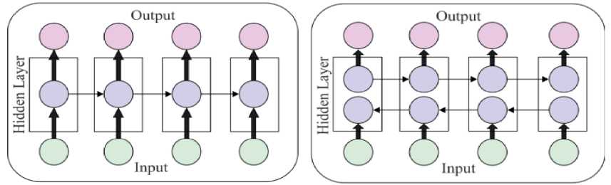
(a) LSTM

(b) BLSTM

Fig. 1. LSTM vs. BLSTM

It facilitates the erroneous signals' passage through the gradient reduction issue. For lingering issues, try constructing a long short-term memory (LSTM) unit with a forgot gate. Important LSTM units are listed below.

First Input: The LSTM unit makes use of the current input vector represented by x_tm and the outcomes determined from the predefining time step represented by h_tm-1 . With tanh activation, the weighted inputs are combined and communicated, leading to z_tm.

This second input gate utilizes sigmoid activation and reads x_tm and h_tm-1 to calculate a weighted total. Thus, it improves the creative outcome by providing input flow into the memory cell.

Forget gate: This gate is a technique from which the LSTM learns to clear the memory of old and irrelevant information. This occurs if and only if the network determines the novel sequence. The forget gate takes in weighted inputs fromx_tm and h_tm-1 and activates them using a sigmoid function. As a result, f_tm is improved by including the state of the cell at the predefining time step, i.e., stem-1, which makes it possible to disregard irrelevant information stored in memory.

The CEC and unit-weighted recurrent edge make up the fourth memory cell. Current cell state s_t . is defined by accepting only relevant data from the most recent input and rejecting any outliers from earlier time steps.

The fifth output gate employs sigmoid activation to manage the outflow of information from the LSTM block and may be utilized with the weighted sum

Sixth Output: An LSTM unit's output, h_tm, is computed by transmitting a cell state c_tm via a tanh and boosting with the next gate, o_tm. Equations are presented that can be used as a guide for implementing an LSTM.

^tm = O(Wi. [Wtm> htm-1] + ^i)(2)

otm P^Wf. [Wtm, htm-1] + ^f)

otm P(^o. [Wtm, htm-1] + ^o)

htm = Otm©tanh(Wtm, CTM)(6)

where i, f, and o are input gates. Now, it represents the sigmoid function used to control input and output information throughout all iterations. Training parameters include "Wi, Wf, Wo, Wc, bi, bf, bo, bc" The outcome at time tm in a bidirectional LSTM not only depends on previous frames in the sequence but also on frames to come. Building a bidirectional RNN, which consists of two RNNs stacked on top of each other, is a breeze. One RNN travels ahead, while the other travels backwards. The mutual result is then subtracted using the RNNs' secret states. Our method employs several LSTM layers, with two LSTM layers used for both onward and reverse permits in the proposed system. In the next part, we'll talk about how IDFOA can help you pick the perfect weight for your BLSTM.

• 4.2.    Hyper-parameter tuning process using IDFOA

• 4.2.1.    Dragonfly algorithm

Both the original and the updated dragonfly algorithms have their foundations laid forth here. Additionally, the updated algorithm flow is shown.

Dragonfly behaviour inspired a new kind of metaheuristic algorithm called the dragonfly algorithm [29]. Separation, alignment, cohesion, foraging, and evasion are the five behaviours seen in dragonfly populations.

The following mathematical models, based on Eqs. (7)-(11) are used to represent these behaviours.

• (1)    The behaviours of evading collisions:

S^-^X-X j                         (7)

where j — 1; 2;... ;N,i — 1; 2;...; Np, N is the amount of people that live in close proximity to one another, and Np is the total population size. If we designate the present person as X, then the jth nearest person's coordinates would be X j .

• (2)    The behaviour of upholding the harmonized group:

  ^A t —

  
  

  у N

  ^ i . " i

  
  
  
  

where V j signifies the velocity of the j th neighbouring separate.

• (3)    The behaviour of touching closer to each other for every separate:

  C_t —

  
  

  v N у

  ^ J=1 ^ i

  
  

  _-

  
  

  N

  
  

  X

  
  
  
  

  • (4)    The behavior of foraging:

  
  

  F_t— X + -X                                         (10)

  
  

  where X⁺ signifies the site of the current separate with optimal value.

  • (5)    The behaviour of eluding opponents:

  
  

  E_t—X + X -                                             (11)

  
  

  where X is the current lowest-fit person in the population.

  Two vectors, step scope (X) and site (X), are added to model dragonfly flying in the search space and allow for location updates. Here is how we calculate the step vector:

  
  

  ^X^⁺¹ — wAX^t + (sS t + uA [ + cC [ + fF [ + eE t )

  
  
  
  

  where s, a, c, f, and e designate the weights of five behaviours, ы is the weight, and t is the current iteration. The position vector is updated as follows:

  
  

  X^t+1 — X^t +AX^t+1

  
  
  
  

  A random walk method is implemented to increase the unpredictability of the search when there are no neighbouring persons. The position vector equation in this scenario is given by Eq. (14):

  
  

  X^t+1 — Levy(d) xX^t +X^t                                (14)

  
  

  where d signifies the dragonfly separate.

  The Levy flight approach is labelled as in Eqs. (15)-(16):

  
  

  Levy(x) — 0.01 x ^—^ \r 2 \P

  
  
  
  

  /               \^1/P

  ra+p—mffi) r^y?*²^

  
  
  
  

• 4.2.2.    Improved dragonfly algorithm

• 4.2.2.1.    Adaptive learning factor

where r1, r2 are two stochastic info in [0,1], b is a continuous, which is occupied as 1.5, Г(х) = (x — 1)!.

This sub-section deliberates the (1) adaptive factor; (2) difference evolution policy; and (3) flow of better procedure.

Dragonflies in the search space are placed there at random. When there are no other particles in the immediate area, the particle in question will randomly wander. When the number of possible iterations is minimal, this circumstance will slow trend and lower the c accuracy. A learning component is implemented to address this concern. And the rate of dragonfly fitness change compared to its initial value is described:

v =

k(X)-H4_es t )l ^{f (} ^ best )+^

The adaptive learning issue of the ith in the tth iteration is spoken as follows:

Ct= —

¹     1+e^-v

When there are adjacent persons around, the sight vector of the ith dragonfly at the tth iteration is described as follows:

X^¹ = C ^ x f + AX^ ¹

Otherwise, the position vector is intended as follows:

X^ = C^x f + Levy(d) x X -                               (20)

• 4.2.2.2.    Differential evolution policy

The search procedure halts when the procedure reaches the local optimum solution. The differential evolution approach is implemented to keep the population diverse and prevent it from converging too quickly. Also, a dynamic scaling factor and the DE/best/1 mutation technique are used. Here is the exact equation:

Н^Х^ + Р^Х^—Х^

where H - is the mutant vector, i = 1,2,..., Np. p 1 , p₂ £ f(1,2, ■■■, Np} are random integers and p 1 , p₂. F f is the scaling factor and can be intended underneath:

гt   17           ( F     _ F      1    f(X i ) f(X best )

^F i     ^r initial ^{+ (r} final    ^r 1n1t1al ). f^t   _t)-f(x^  )

where F_1n1t1al and F f _1nal are two constants (X ,w _Ors) is the worst fitness value amongst the population in the t th repetition. After obtaining the distorted vector, the crossover process is achieved to yield a trial vector У ] = (У -! , V^,...., V^using

Eq. (23):

^V ] = {

Hi ]   if j = j0 and rand(0,1) < pCR

X t           else

where j = 1,2, .,d,j₀ £ {1,2, .,d} is a random dimension, pCR characterizes cross likelihood within the range of [0,1].

In conclusion, the population is efficient by comparison the fitness value. The assortment strategy is exposed as follows:

t₊i  (V? iff(V^

• ¹       [X-      else

• 4.2.2.3.    The flow of enhanced dragonfly procedure

The exact stages of IDA are portrayed as follows:

• 1)    Tweaking the settings. Limit the sum of repetitions, the particle size, the population size, and the particle bounds.

• 2)    Set the initial values for the location and step vectors.

• 3)    Begin iterating. Check the population's fitness levels, and remember to update the weight coefficient. Then, adjust where the resources and danger are located.

• 4)    Use Eqs. (7)-(11) to revise the values of S,A, C, F, and E, and Eq. (12) to revise the step vector. If the present person has no neighbours, then the location may be updated using Eq. (20). Otherwise, the location would be updated with Eq. (19).

• 5)    Apply the differential evolution method to each person by solving Equations (21)–(24).

• 6)    Determine if the termination condition has been met. If this is the case, you should halt the iteration and provide the output. If not, go back to the third step.

5.    Results and Discussion 5.1.    Network Setup

The optimization skills of IDFOA are put to the test by applying it to a collection of classical functions. Two unimodal functions and three multimodal functions are found in the first set. Table 5 displays detailed information on dimensions, including the ideal value and domain.

Table 5. Parameter settings of dissimilar procedures.

Algorithm	Sum of max iterations	Size of population
	500	40
IDFOA	levy flight continual	inertial weights
	1.5	[0.9,0.4]
DA	levy flight continual	inertial weights
	1.5	[0.9,0.4]
PSO	C1	C2
	1.49445	1.49445

To prevent unfair comparisons of performance during training, K-fold cross-validation (K = 4) was used to objectively assess the efficacy of the changed procedures across the two groups (shallow and deep). Several low-power systems now have the intended application running on them.

Table 6. Experimental Analysis of proposed model on various cases

Experimental Cases	MAE	R2	RMSE	MAPE (%)
Case-1	0.274	0.685	0.469	31.42
Case-2	0.260	0.724	0.445	31.73
Case-3	0.262	0.719	0.447	31.64
Case-4	0.225	0.785	0.388	28.33
Case-5	0.262	0.715	0.452	31.52

The experimental analysis of the model's suggested assumptions in various cases is shown in Table 6 above. The RMSE value was 0.469, the MAE value was 0.274, the MAPE value was 31.42, and the R2 value was 0.685 in the analysis of Case 1, respectively. Another Case 2 condition had RMSE values of 0.445, MAE values of 0.260, MAPE values of 31.73, and R2 values of 0.724, respectively. In a different Case 3 scenario, the RMSE value was 0.447, the MAE value was 0.262, the MAPE value was 31.64, and the R2 value was 0.719. Another Case 4 condition had RMSE values of 0.38, MAE values of 0.225, MAPE values of 28.33, and R2 values of 0.785, respectively. In a different Case 5 scenario, the RMSE value was 0.452, the MAE value was 0.262, the MAPE value was 31.52, and the R2 value was 0.715, respectively.

Table 7. Conditions the RMSE value as: Statistical material of output data of LSTM, BLSTM and proposed BLSTM-IDFOA.

Methods	Strokes	RMSE	MAE	MAPE (%)	R2
BLSTM-IDFOA	Basic	35.66	19.35	50.58	0.835
	Top	44.21	24.75	54.64	0.808
	Push	34.25	19.71	45.28	0.862
BLSTM	Basic	47.67	26.14	99.07	0.642
	Top	58.68	36.12	73.64	0.703
	Push	48.03	29.28	69.64	0.724
LSTM	Basic	44.23	26.46	177.52	0.247
	Top	66.08	43.41	94.59	0.463
	Push	47.71	29.44	88.66	0.429

In Table 7, the RMSE value is represented as the statistical material of LSTM, BLSTM, and the proposed BLSTM-IDFOA output data. Different methods are used in this analysis to compare the various models. The RMSE value for the basic stroke in the BLSTM-IDFOA method was 35.66, the MAE value was 19.35, the MAPE value was 50.58, and the R2 value was 0.835. And BLSTM in the top stroke, as the RMSE value was 44.21, the MAE value was 24.75, the MAPE value was 54.64, and the R2 value was 0.808. And the RMSE value for the push stroke was 34.25, the MAE value was 19.71 45.28, and the MAPE value was 0.862. And the RMSE value for the basic stroke was 47.67, the MAE value was 26.14, the MAPE value was 99.07, and the R2 value was 0.642. And in the top stroke, the RMSE value was 58.68, the MAE value was 36.12, the MAPE value was 73.64, and finally the R2 value was 0.703. And the RMSE value for the push stroke was 48.03, the MAE value was 29.28, the MAPE value was 69.64, and the R2 value was 0.724. And in the LSTM model, the RMSE value for the basic stroke was 44.23, the MAE value was 26.46, the MAPE value was 177.52, and the R2 value was 0.247. And in the top stroke, the RMSE value was 66.08, the MAE value was 43.41, the MAPE value was 94.59, and the R2 value was 0.463. And the RMSE value for the push stroke was 47.71, the MAE value was 29.44, the MAPE value was 88.66, and the R2 value was 0.429, respectively.

6.    Conclusion

Growing quantities of high-quality sports video data are becoming increasingly important for tracking players and other actions in broadcasts. Therefore, there is both theoretical and practical utility in employing a computer's extensive memory and processing ability to identify and comprehend video content. Therefore, the primary objective of the authors is to create a teaching plan. The system can tailor lessons for individual players, making it ideal for teaching newcomers. As the third stage of the system, the suggested BLSTM based on IDFOA was implemented to approximate the quality scores of the table tennis strokes performed using the study's five assessment criteria. The major goal of this research was to apply both technical and functional criteria to the evaluation of the three forehand varieties used in table tennis (basic, topspin, and push). BLSTM-IDFOA method was 35.66, the MAE value was 19.35, the MAPE value was 50.58, and the R2 value was 0.835. And BLSTM in the top stroke, as the RMSE value was 44.21, the MAE value was 24.75, the MAPE value was 54.64, and the R2 value was 0.808. And the RMSE value for the push stroke was 34.25, the MAE value was 19.71, 45.28, and the MAPE value was 0.862. The sensing modality of object sensors was employed in this work to construct the data-gathering tool because of its applicability.

The study also had a practical component in that the coaching group involved in it manually scored and labelled the quality of the strokes that were executed. Moreover, from a technical standpoint, it is essential that the suggested Forehand quality estimate models produce accurate predictions. The shadow-play support solution would be too expensive to implement due to the sensor modalities. The chosen sensing modality for the object sensors is low-cost, highly flexible, and user-friendly; these qualities combine to make the proposed method simple to implement. In this study, data was collected using a racket integrated with an IMU, which ensured the players' privacy (at least from outside observers) and anonymity.

7.    Future Work

Future development might involve integrating Cloud Internet Services with the virtual-coach table tennis training scheme to keep track of the player's practice history for the next stage of endorsements and feedback. In addition, if players coach, it may be combined with requests to display graphical and visual feedback to coaches. The automated analysis of strokes and comments provided over time might lead to performance improvement rates for the players. The method would help players improve their skills without a coach by teaching them table tennis shadow play on their own and giving them relevant automated feedback.