Exact solutions of the (2+1)-dimensional Kundu-Mukherjee-Naskar model via IBSEFM

Various natural phenomena in physics are modelled by nonlinear partial differential equations. Investigating the exact solutions of these equations is very important to describe the nonlinear physical process ranging from graviation to fluid dynamics. Models of real-life problems such as nonlinear waves [1], temporal transitions [2], shallow water waves [3] and plasma physics [4] are based on nonlinear phenomena. For a better understanding of these equations, many p owerful methods were introduced by mathematicians for exact solutions of nonlinear partial differential equations. Some of them are the Adomian decomposition [5], (G' /G)-expansion [6], the improved tanh function [7], IBSEFM [8], extended direct algebraic method [9] and others.

In recent years, a deep research attention was paid to rogue wave solutions. Recently, in [10], a new completely integrable (2+1)-dimensional nonlinear evolution equation was derived to describe the dynamics of two-dimensional oceanic rogue wave phenomena. In the paper [10], this nonlinear dynamical equation was called the Kundu-Mukherjee-Naskar (KMN) equation. Firstly, the rogue waves were observed in the deep oceans and then derived in modelling nonlinear ion acoustic waves in magnetized plasma system [11]. In literature, there exist only four methods to find exact solutions of (2 + 1)-dimensional KMN equation. These methods are trial equation method [12], extended trial function method [13], traveling wave reduction [14], extended direct algebraic method [15].

In this study, we consider the following (2+1)-dimensional KMN equation:

iu t + a ₆ u xy + ia ₇ u(uu X — u * u_x) = 0,                         (1)

where i = д/ — 1, u(x,y,t) represents the nonlinear wave function with the independent variables x, y (space coordinates) and t (time), u ^∗ denotes complex conjugation of u . Here, the coefficient α 6 is the dispersion term and the coefficient α 7 is the nonlinearity term. Before beginning of the solution procedure, we should describe the proposed method.

1.    Description of IBSEFM

In this section, we give the fundamental properties of the IBSEFM [8]. Let us present the five main steps of the IBSEFM [16–20].

Step 1. Consider the following nonlinear partial differential equation in two independent variables x and t:

P (u, u t , u xx , ...)    0,

where P is the function containing u, u _t , u _xx , ... and the subscripts denote the partial derivatives of u(x,t) with respect to x and t. The aim is to convert (2) into the ordinary differential equation with a suitable wave transformation as

u(x,t) = V К), € = X - pi-

Using (3), equation (2) turns into the ordinary differential equation of the form

N (V,V ‘ ,V ‘‘ ,...) = 0,                                   (4)

where N is the function of V and its derivatives V ^′ , V ^′′ , ... with respect to ξ . If we integrate (4) term by term, we obtain integration constants which can be determined later.

Step 2. Hypothesize that the solution of (4) can be presented as follows:

n

E a i F i«) v (€) = .--------

E j f j (€) j=0

a o + a i F (€) + a 2 F ² (€) + ••• + a n F ⁿ (€) b o + b 1 F (€) + b ₂ F ²«) + ... + b m F ^m«) ’

where a ₀ , a 1 ,..., a_n and b ₀ , b 1 ,..., b_m are coefficients to be determined later, m = 0,n = 0 are chosen arbitrary constants of the balance principle, and the form of Bernoulli differential equation is as follows:

F ‘«) = aF (€) + dF M (€), d = 0, a = 0, M G R / { 0,1, 2 } ,             (6)

where F (€) is a polynomial.

Step 3. The positive integers m, n, M are found by balance principle that is both nonlinear term and the highest order derivative term of (4).

Substitute (5), (6) in (2) and obtain the equation of polynomial 0(F ) of F as follows:

0(F «)) = PsF (€ )s + - + PiF (€) + Po = 0, where ρi are coefficients to be determined later.

Step 4. The coefficients of 0(F (€)), which give us a system of algebraic equations, turned out to be zero:

p i = 0, i = 0,.., s.

Step 5. When we solve (4), we get the following two cases with respect to σ and d:

F (€) = [

- de^ ^-1 + ae⁰"^^-1^

■ ] ^1-‘ ,

d = a,

F «) =

— 1) + (e + 1) tanh(a(1

1 — tanh ( a(1 — e) 2

)--— j ,d = a, e E R.

Using a complete discrimination system for the polynomial of F (£), we obtain the analytical solutions of (4) via mathematics software and categorize the exact solutions of (4). To achieve better results, we can plot two and three dimensional figures of exact solutions by considering proper values of parameters.

2.    Application of IBSEFM

In this section, the application of the IBSEFM to the KMN model is presented. Let us consider the following wave transform:

u (x,y,t) = U «) e^ytt,(9)

where U (£) represents the amplitude portion and

£ = a1x + a2 y — nt,(10)

and the phase portion of the solution is defined as

ф(x,y,t) = —a3 x — a4y + a51.(11)

Then, we get the nonlinear ordinary differential equation ai a%a6U — (a5 + аза4аб )U — 2аза7 U3 = 0,(12)

П — —аб(а2аз + ai a4).(13)

Then we reconsider (12) for the balance principle considering among U ^′′ and U ³ and get the relationship as follows:

M = n — m +1.(14)

Formula (14) shows different cases of the solutions of (1) and we can obtain some exact solutions. According to the balance, we consider M = 3,m = 1,n = 3 for (12) and (14), and the following equations hold:

and

U "(£) =

u (£) =

a o ⁺ a i G ^{( £} ) ⁺ a ₂ G ^{2 ( £} ) ⁺ a 3 G³U ) _ T ^{( £} )

и ‘ (£) =

b o + b i G(£ )                Ф(£ )’

T‘«)Ф (£) — Т«)Ф ‘ (£)

ф²« )

,

T ‘« )Ф ( £ ) — T«)Ф ‘« )   [T«)Ф ‘ ( £ )] ‘ Ф ²« ) — 2T«)[Ф ‘« )] ² Ф«)

Ф2«)

—

W)

,

where G' = aG + dG³, a ₃ = 0, b 1 = 0, a = 0, d = 0. Using (15)-(17) in (12), we get from the coefficients of the polynomial of G the following:

Constant : — a 0 b 0 a ₅ — a ₀ b 0 a ₃ a ₄ a ₆ — 2a 0 a ₃ a 7 = 0,

G : — a 1 b 2 a ₅ — 2a ₀ b ₀ b 1 a ₅ — a 1 b 0 a ₃ a ₄ a ₆ — 2a ₀ b ₀ b 1 a ₃ a ₄ a ₆ + a ² a _i b 0 a 1 а ₂ а ₇ —

• — 6a 0 a 1 a ₃ a 7 = 0,

G² : a 2 b 2 a 5 — 2a i b o b i a 5 — a o b O а з a 4 a6 — a 2 b 0 а з а 4 аб — 2a i b o b i а з а 4 аб —

— a_ob² a ₃ a ₄ a ₆ + 4a ² a ₂ b 2 a 1 a ₂ a ₇ + a ² a ₀ b ^ а 1 а ₂ а ₇ — 6a _o a 1 а ₃ а ₇ — 6a 2 a ₂ a ₃ a ₇ = 0

G ³ : — a ₃ b 2 a ₅ — 2a ₂ b ₀ b 1 a ₅ — a1b²a ₅ — a ₃ b 2 a ₃ a ₄ a ₆ — 4daa ₀ b ₀ b 1 a ₁ a ₂ a ₇ —

• — a 1 b 2 a ₃ a ₄ a ₆ + 4daa ₁ b 0 a ₁ a ₂ a ₇ — 2a ₂ b ₀ b 1 a ₃ a ₄ a ₆ + 9a ² a ₃ b 0 а 1 a ₂ a ₇ +

+3a 2 a 2 b o b i a i a 2 a 7 — 2 а 3 а з а 7 — 12a o a i a 2 a 3 a 7 — ба О а з а з а 7 = 0,

G 4 : —2a 3 b o b i а 5 — a 2 b²a5 — 2а з b o b i а з а 4 а б — a 2 b²a з a 4 a 6 + 12daa 2 b 2 a 1 a 2 а 7 — + 11a ² a ₃ b ₀ b1a ₁ a ₂ a ₇ + a²a₂b² а 1 а ₂ а ₇ — 6a ² а ₂ а ₃ а ₇ — 12a ₀ a ₂ а ₃ а ₃ а ₇ = 0,

G ⁵ : — a ₃ 1га 5 — а₃Ь²а ₃ а ₄ а ₆ + 3d ² a 1 b 0 a 1 а ₂ а ₇ + 24daa ₃ b 0 а 1 а ₂ а ₇ — 3d ² a ₀ b ₀ b ₁ a ₁ a ₂ a ₇ +

• — +12daa 2 b o b i a i а 2 а 7 + 4а ² а з b ² a i a 2 a 7 — 6а 1 а 2 а з а 7 — 6а ² а з а з а 7—

• —    12a o a 2 а з а з а 7 = 0,

G ⁶ : 8d ² a ₂ b o a _i a ₂ a ₇ + d ² a _i b _o b _i a _i a ₂ a ₇ + 32daa ₃ b ₀ b ₁ a ₁ a ₂ a ₇ — d²a_ob²a _i a ₂ a ₇ +4daa ₂ bl a _i a ₂ a ₇ — 2а 2 а _з а 7 — 12a _i a ₂ a ₃ a ₃ a ₇ — 6a _o a 2 a ₃ a ₇ = 0,

G 7 : 15d 2 a 3 b 2 a i a 2 a 7 + 9d ² a 2 b o b i a i a 2 a 7 + 12daa з b 1 a i a 2 a 7 — 6a 2 а з а з a 7—

• — 6a i a 2 a з a 7 = 0,

G 8 : 21d ² a ₃ b _o b _i a _i a ₂ a ₇ + 3d ² a ₂ b 2 a _i a ₂ a ₇ — 6a ₁ a 2 a ₃ a ₇ = 0,

G ⁹ : 8d ² a з b 1 a i a 2 a 7 — 2а з а з а 7 = 0.

By solving the above system, we obtain the coefficients as follows.

Case 1. For a = d, we can consider the following coefficients obtained by a software:

a 0

. С а з ^ 0₄ ^ o 6 b_o

α 3 α 4 α 6 b 1

i /— , J— ; v 2 д/аз ^/07

—i— — /— — /— —; a i = — V 2 д/аэ ^/57

—i д/2 d C a з a 4 а б + а 5 b o      —i д/2 d C a з a 4 a 6 + а 5 b i

-------г- -------; ^аз =-------------- α ₃ α ₇ σ                    α ₃ α ₇ σ

Substitute these coefficients along with (7) in (15) and obtain the complex solution of (1):

—^-(-zt+^y^

v^² С ° з V ° 7

where α ₂ , α ₃ , α ₆ , α ₇ , σ are not equal to zero.

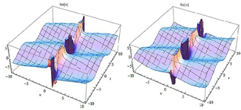
Fig. 1 . 3D-plots of u 1 (x,y,t) for the values d = 0,4; a = 0,4; a ₂ = 0,9; a ₃ = 0,5; a ₄ = 0, 3; a ₅ = 0, 25; a ₆ = 0,1; a ₆ = 0, 7; a ₇ = 0, 3; e = 0, 2; - 15 15, - 15 15

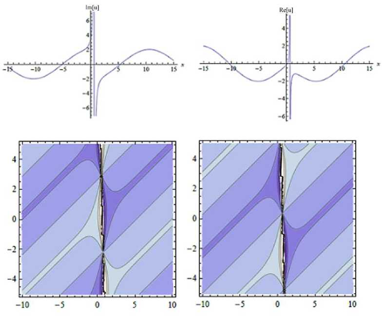
Fig. 2 . 2D-graphs of

u 1 (x,y,t) for - 15 < x < 15, t = 0,1 and contour surfaces for

- 10 < t < 1

Case	2. For a = d, we consider the following coefficients obtained by a software: _   y a i ^ a 2 y a 6 ab o       / a l / a 2 / a 6 ab 1 a 0                --- --- ; ai              --- --- ; α 3 α 7                   α 3 α 7 2d / a i / c ^ / c ^ ab i          a 5 + 2a 1 a 2 a 6 a 2 аз —             ___ ___ ; a'4 —                       . α 3 α 7                       α 3 α 6
Substitute	these coefficients along with (7) in (15) and obtain the complex solution of (1): /                                         \
u 2	_________________-_____2d + a I | 2ст ( а1 a5-a2a3аб + 2а1 а2аб^2 ) t + aia3x + a2a3y |               1 exp -                      α3                        ǫ- σ d (x,y,t) =                /-------   ^r-             X v — c a c ac*+ + ааз ya ? ie^ a s t - a s x ) /— a 1 a 2 a 6 X /--------, r- ^’ v —ai a 2 a g + а^з ya?
where α 1 ,	α 2 , α 3 , α 6 , α 7 , σ are constants different from zero.
-10/ if
-it
-10	10
Fig. 3 . 3D a 5 = 0,1;	)-plots of u 2 (x, y,t) for the values d — 0, 5; a — 0,4; a 3 — 0, 2; a 4 — 0, 8; a 6 — 0, 7; e — 0,1; — 10 < x < 10, — 10 < t < 10
Case	3. For a — d, /—а з а 4 аб — a 5 a 2          —/—а з а 4 аб — a 5 a 2 b i         a 2 b i
a 0	2V2d / a 1 / a 2 2V2d / a i / a 2 ^bo ’        bo ’ 4d 2 aia 2 a 6 b 2           X—a 3 a 4 a 6 — a 5
α7	2        ; a                                   . a 3 a 2             v2 y/ai у«2 v/«6

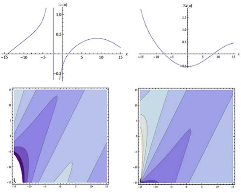
Fig. 4 . 2D-graphs of u ₂ (x,y,t) for - 15 < x < 15, t = 0,2 and contour surfaces for

- 15 < x < 15, - 15 15

Substitute these coefficients along with (7) in (15) and obtain the complex exponential function solution as follows:

U 3 (x,y,t) =

X

/

| 2a ( ^a i ^a 5 ^-. exp -

2d а2а3аб+2а1 a2a6^2)t + aia3x + a2a3y

α3

d α 1 α α 6 +b ² ₀

² ^^3 V-^a3 ^a 4 ^a 6 — ^a5\/ --ZZ^---

α 3 a ₂

_ie -i(α 5 t+α 3 x+α 4 y)

v^al У«2 д/аё д/a ₃ a ₄ a ₆ + a ₅

²^ ^а з ^- о З д ^ й б

-

α 5

d ² α 1 α 2 α 6 +b ² ₀ α 3 a ² ₂

ǫ- σd

X

where a 1 , a ₂ , a ₃ , a ₆ , a ₇ , a = 0.

Conclusion

In this work, the Improved Bernoulli Sub-Equation Function Method (IBSEFM) is used in (2+1)-dimensional Kundu–Mukherjee–Naskar (KMN) equation. Various solitary wave solutions are successfully constructed. Using mathematics software, two and three dimensional figures and contourplot surfaces of the solutions are plotted according to the suitable values of parameters. According to the results, we see that the formats of travelling

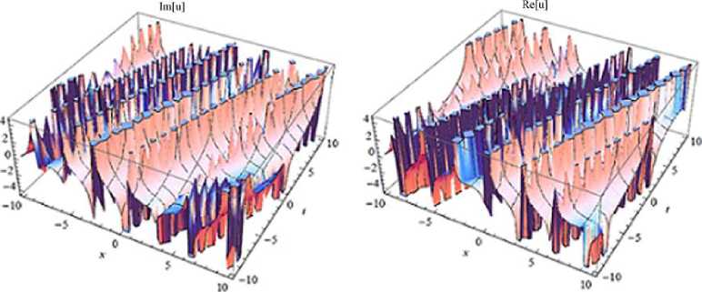
Fig. 5 . 3D-plots of u ₃ (x,y,t) for the values d = 0,3; a = 0,4; a 1 = 0,6; a ₂ = 0,5; a ₃ = 0, 2; a ₄ = 0,1; a ₅ = 0, 9; a 1 = 0, 3; a ₇ = 0,1; e = 0,1; - 10 < x < 10, - 10 10

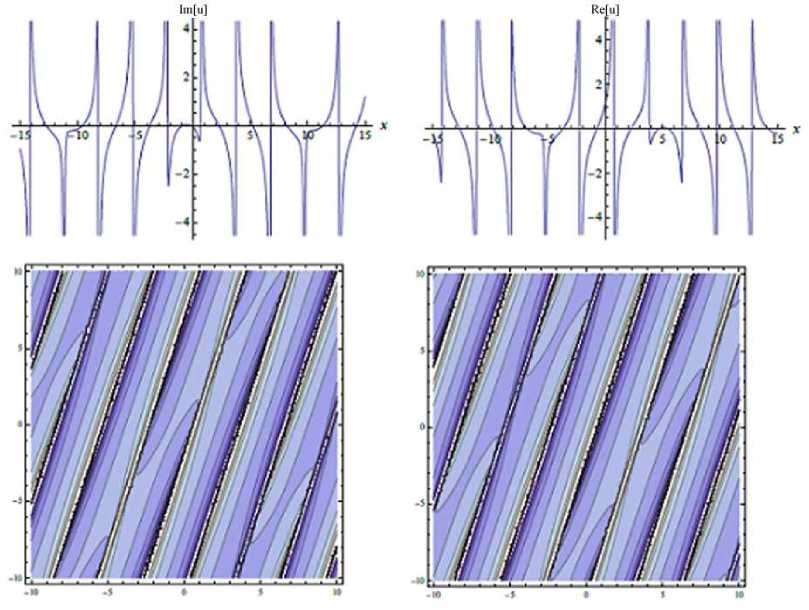
Fig. 6 . 2D-graphs of

u ₃ (x,y,t) for - 15 < x < 15, t = 0,3 and contour surfaces for

- 10 < x < 10, - 10 10

wave solutions in two and three dimensional surfaces are similar to the physical meaning of results. The solutions are also solitary wave solutions. It is also clear that the more steps are developed and the better approximations are obtained. The conclusions show that the IBSEFM is simple, effective and p owerful. Therefore, the IBSEFM is applicable to solve different kind of nonlinear partial differential equations in mathematical physics.