Existence of lower and upper solutions in reverse order with respect to a variable in a model of acidogenesis to anaerobic digestion

Anaerobic digestion (AD) is a microbial fermentation in the absence of oxygen results in a mixture of gases (mainly methane and carbon dioxide), known as "biogas" and an aqueous or "sludge" suspension containing the microorganisms responsible for degradation of organic matter. The raw material used primarily to be subjected to this treatment is any residual biomass that has a high moisture content, such as food scraps, leftover leaves and herbs to clean up a garden or orchard, livestock waste, sludge treatment plants urban wastewater and domestic sewage and industrial.

In practice, engineering becomes accustomed to consider three stages for solid waste or sludge (hydrolysis, acidogenic, methanogenic) and two for liquid waste (acidogenic and methanogenic) [1].

We consider the following system of nonlinear ordinary differential equations for the process AD [2]:

Balance of biomass

	dX 1 dt dX 2 dt	= ( A 1 ( S 1) — aD ) X 1 = ( A 2 ( S 2) — aD ) X 2	(acidogenic) (metanogenic)	(1) (2)
Balance of substrates
dS 1 dt	= D ( S 1 in -	S 1) - k 1 A 1( S 1) X 1	(acidogenic)	(3)
dS 2 dt	= D ( S 2 in -	S 2) + k 2 A 1( S 1) X 1 —	k 3 A 2( S 2) X2 (metanogenic)	(4)

M.M. Higuera, A.V. Sinitsyn

Balance of alkalinity

_dt = D ( Ai_n - A )

Carbon rate of change

—- = D ⁽ Cin ^— C ) + к 4 Ц 1⁽ S 1) X 1 + к 5 Ц 2⁽ S 2) X 2 ^— KL a ^[ C + S 2 ^— A ^— KHPC ^] .    (6)

The expression KLa ( C — KH PC ) describes the molar flow rate of inorganic carbon from its liquid phase to its gas phase and the product KH PC determines the concentration of dissolved oxygen in C.

Net rate of methane production dFM dt

= k 6 µ 2 ( S 2) X 2 .

The kinetic comportment is nonlinear and occurs because of reaction rates, which are given by: Monod kinetics ц 1( S 1) = ц 1 max „ S b, and Haldane kinetics ц ₂( S2) = S 1 + K S ₁

ц2max"^ 2— S ²----• Bacterial rate represents yield related to both bioprocesses.

_K ^S _I ²₂+ S 2+ K S ₂

In this case the variables are:

S ₁ := Organic substrate concentration [g / l]

X 1 := Concentration of acidogenic bacteria [g / l]

S ₂ := Volatile fatty acids concentration [mmol / l]

X 2 := Concentration of methanogenic bacteria [g / l]

A := Concentration of alkalinity [mmol / l]

C := Total inorganic carbon concentration [mmol / l]

FM := Methane concentration [mmol / l d ^{- 1}] .

The main objective is to build lower-upper solutions for the system formed by equations (1) and (3) in reverse order with respect to a part of variables with initial conditions on a given observation interval [3].

The corresponding ecpiations:

u^′ = f ( x, u, v ) in I, v^′ = g ( x, u, v ) in I,

where I = [ a,b ] u = X 1, v = S 1. Note that the definition of lower-upper solution (8) depends greatly on the properties of monotony of f and g. Therefore following notation of C.V. Pao in [4] and new results presented in [5], we can classify (8) according to their relative monotony, as follows:

• 2.    Mixed quasi-monotone systems: either, f is nondecreasing in v and g is nonincreasing in u. or vice versa.

• 3.    Nonquasi-monotone systems: the system does not fall in any of the previous cases.

Case 1 implies the existence of lower ( u*,v* ) and upper ( u*,v* ) solution with ordering in I

• u∗ ≤ u^∗ ,    v∗ ≤ v^∗ .

It is impossible to enforce cpiasi-monotonicity by a simple transformation for Case 2. Case 3 requires some regularity conditions imposed on f and g.

In the above system, the usual order ( X 10 < X 0) is considered for the lower and upper solutions. For the variable S 1 the situation is different because of the opposite case S 0 < S io- We consider the nonlinear equation [6]

u ( t ) = f ( t,u ( t )) , t E I = [0 ,T ] , T> 0                      (9)

satisfying the condition [6]

g ( u (0) ,u ( T )) = 0 ,                                   (10)

where f : I x R ^ R and g : R2 ^ R are continuous functions. If g(x,y) = x — c with c E R, then (10) is the initial condition u (0) = c.

Definition 1. [6]

e w E C 1(I) is a lower solution to (9) if w' (t) < f (t,w (t)), t E I and w (t) < в (t), t E I                                 (11)

e в E C 1(I) is upper solution to (9) if в'(t) > f (t,e (t)), t E I and в (t) < w (t), t E I                                 (12)

For u,v E C ( I ). u < v define the set

[ u,v ] = {Vw E C ( I ) : u ( t ) < w ( t ) < v ( t ) , with t E I}.

Definition 2. [6] We say that ш,в E C 1(I) are lower and upper coupled solutions to problem (9), (10) in direct order if w is a lower solution and в is an upper solution to equation (9), with condition (11) and max{g(w(0) ,w(T)) ,g(в(0) ,в(T))} < 0 < min{g(в(0) ,в(T)) ,g(в(0) ,w(T))}.

M.M. Higuera, A.V. Sinitsyn

Definition 3. [6] We say that ш,в G C 1(I) are lower and upper coupled solutions to problem (9), (10) in inverse order if ш is a lower solution and в Is an upper solution to equation (9), with condition (12) and max{g(ш(0),ш(T)),g(в(0),ш(T))} < 0 < min{g(в(0),в(T)),g(ш(0),в(T))}.

Theorem 1. [6] It is assumed that ш,в o,re lower and upper solutions coupled in inverse order to problem (9), (10). Additionally it is assumed that the functions hш(x) := g(х,ш(T)),   he := g(х,в(T))

are monotonic (both non-increasing or non-decreasing) in [ в (0) , ш (0)]. Then there exists at least one solution of problem (1) - (3) in [ в,ш ].

The inverse order of lower and upper solutions for system (1) - (7) were not previously considered. The outline of this paper comprises the following stages: definition of trivial solutions for the complete system, construction of lower and upper solutions for a subsystem, study and formulation of the corresponding theorem for the existence of lower and upper solutions.

Definition 4. A trivial solution of system (1) — (7) has the form

E i( S i in, 0) , E 2( S i in, 0 ,S 2 in, 0) , E 3(0 , 0 ,S 2 in ) E 4( S 1 in, 0 ,S 2 in, 0 ,Ain ) , E 5( Ain ) , E б(0 ,S 2 in, 0)

where

X 1 = 0 , X 2 = 0 , S 1 = S 1 in

^S 2 = ^S 2 in, A = Ain, ^C = Cin, FM = ⁰

We do not consider other possibilities of trivial solutions in this document. A similar approach can be found in [7].

1.    Main Results 1.1.    Lower and Upper Solutions to the Initial Value Problem

We are interested in solutions of nonlinear system with initial conditions, which models the dynamics of biomass and substrate in the acidogenic.

dX1

, F ( t,X 1( t ) ,S 1 ( t )) ,

(14a)

dt    V1   S1 + Ks 1      / dS1 = D (S1 in — S1) — k 1 ц 1 max q S'    X1       , G(t,X 1(t), S 1(t)),      (141.))

dt                             S 1 + Ks 1

X 1(0) = c1,(14c)

S 1(0) = c2.(14d)

Where t G [0 ,T ] = I . with T >  0 arid F,G are functions of class C ⁰( I ) = C ( I ). i.e.. continuous functions in I.

A. Define

SS f ^{( S} 1) = Ц 1 m        _к --^aD and g ⁽ S 1) = Ц 1 max           .

S 1 + K s i                             S 1 + K s i

The function g ( S 1) = ц 1 max S 1 + SK S with ц 1 _max ,K_S 1 >  0 is a monotonically increasing function such that g ( S 1) — > ц 1 _max as S 1 —> to.

If Ц 1 max s Sк --aD >  0 then it can be proved that f ( S 1) = O ( g ( S 1)), i.e., ^max S 1 + K_{S 1}

V ( S 1) 3 ( c> 0) such that ||f ( S 1) || < cig ( S 1) ||.

⁰ < ^Ц 1 max

S 1

S 1 + ^KS 1

-

αD ≤

^µ 1 max

S 1

^S 1 + ^KS 1

S 1

max S 1 + K s 1

-

αD

< 1

^µ 1 max

S 1

^S 1 + ^KS 1

= ^|f ( S 1) |< c lg ( S 1) ||

^µ 1 max

S 1

^S 1 + ^KS 1

- αD

≤ K.

^If Ц 1 max _S 1 + K _S 1 “ ^aD<  ^{0 theU X} 1 -- ^ ^{0 M1(l}

S 1

^{Ц 1} max S 1 + K s 1

- αD

∥ X 1 ∥ ≤ K.

Condition A shows that the norm

S 1

^{Ц 1} max S 1 + K s 1

- αD

is bounded.

We define the lower-upper solution in inverse order with respect to the variable S 1 and in direct order for X 1 as follows:

Definition 5. [Lower-upper solution] A pair [( X ₁₀ , S ₁₀) , ( X 0 , S 0)] is called

• (a)    a lower-upper solution of problem (14), if the following conditions are satisfied

  ( X 10 ,S 10) G C 1( I ) ,	( X 0 ,S 0) G C 1( I ) ,	t ∈ I
  XX 10 _ F ( t, X 10 , S 1) <  0 XX 10 - F ( t,X 0 ,S 1) >  0 in	I, VS 1 G [ S 0 ,S 10] ,	(lower)                     (15a) (upper)                     (15l>)
  ^S10 — G ( t, X 1 , S 10) <  0 S 0 — G ( t,X 1 ,S 0) >  0 in	I, VX 1 G [ X 10 ,X 0]	(lower in inverse order) (15c) (upper in inverse order) (15d)
  with X 10(0) < c 2 < X 10(0) ,	S 10 (0) < c 1 < S 10 (0)	(initial conditions);       (15e)

M.M. Higuera, A.V. Sinitsyn

• (b)    a lower-lower solution of problem (14), if the following conditions are satisfied

X 10 ^— F ^{( t,X} 10 , S io) <  ⁰ in I,

So — G(t, X10, S10) < 0 in I with S0(0) < c 1 < Sю(0);

(c) an upper-upper solution of problem (14), if the following conditions are satisfied

X0 - F(t,X0,S0) > 0 in I, S0 - G(t,X0,S0) > 0 in I with X10 < X°,  S0 < S10 in I.

Definition 6. The functions Ф( t,ts 1 i,E 1 max ,K s 1 ,D,a ), Ф1( t,tx 1 i,D,S 1 in,k 1 ,p 1 max,Ks 1) are called semitrivial solutions of problem (14)

if Ф( t, t_S 1 i ,p 1 _max,K_S 1 ,D,a ) is a solution of the ODE:

У                 tSu---

1      M1 max .     , tS 1 i + KS1

- αD X 1

and Ф1( t, t_x 1 i,D,S 1 _in,k 1 , m 1 max,KS 1 ,a ) is a solution of the following ODE:

S 1 = D ( S 1 in

-

^S 1) + k 1 E 1

max

S 1

S 1 + K s 1

^tX 1 i^.

Here t_S 1 i ,i = 1 , 2 , 3 a nd t_x 1 i ,i = 1 , 2 , 3 are the indicators of semitrivial solutions Ф( t,ts 1 i,E 1 max,Ks 1 ,D,a ) ЫФ1( t, tx 1 i,D,Sin,k 1 ,M 1 max,Ks 1) respectively, defined by the. following way:

If S 1 = S 1 in. then ts 11 = S 1 in

If S 1 = S ⁰, then t_S 12 = S ° is an upper solution of problem (17);

If S 1 = S ₁₀, then t_{S 13} = S ₁₀ is a lower solution of problem (17);

If X 1 = 0. then tx 11 = 0:

If X 1 = X^, then t_x 12 = X ⁰ is an upper solution of problem (16);

If X 1 = X ₁₀, thicn t_{x 13} = X ₁₀ is a lower solution of problem (16).

From Definition 6, we obtain different types of semitriviales solutions of system (14):

XX 1 = (,

S 1 in µ 1 max

S 1 in + KS 1

-

αD X 1 ,

S 1 = D ( S 1 in - S 1)

(18a)

(18b)

for ( X 1 , S 1) with ordering of lower and upper solution

X 10( t ) < X 1⁰( t ) ,   S 1⁰( t ) < S 10( t ) .

Theorem 2. Assume that condition A is fulfilled and there exists a pair (X10, Sf), (X0, S10) of lower-upper solutions of (14). Then there exists at least a solution of semitriuial equations (16), (17) and there exists a solution (X 1, S 1) of system (14) such that

X io ( t ) < X 1( t ) < X 0( t ) ,     t E I

S 0( t ) < s 1 ( t ) < s 10 ( t ) ,       t E I.

Proof. It is divided into two steps. First, we consider a modified problem and show that any solution of this problem is also a solution of the original problem and that it is between X ₁₀ and X ⁰, S 0 and S ₁₀ (reverse order) by means of differential inequalities. Second, a direct application of the Banach fixed point theorem shows that equations (16), (17) for the semitrivial solutions have at least one solution. Last result guarantees the existence of solution ( X 1 , S 1) to system (14).

Step 1. Introduce the space

K = [ X 1o , X °] x [ S О , S 10] c E = C ( I ) x C ( I ) .

K is a bounded closed convex set in E. Now, given ( X 1 , S 1), define the functions:

Г F(t,X0)+ X0 if X10 < u, f(X i,Si)(t,u ) =    F(t,u)+ u if X10 < u < X10 , (20) I F(t,X 10)X10 if u < X10 , Г G (t, S 0) — S 0 if S10 > v, g ( x i ,si)( t,v )=    G(t,v) — v if S10 < v < S10 , (21) [ G(t, S10) — S10 if v > S10. Define the mapping T : K ^ E by T(X 1, S 1) = (u,v) . where u and v are the solutions, respectively, of the modified problems

• ⁽ I )      u ⁽ t ) + u ⁽ t ) = ^f ( x i ,S i)^{( t,u (} t )) ,

u (0) = c 1 ,

• ⁽ II )      v ⁽ t ) - v ⁽ t ) = g ( x i ,s i)^{( t,v (} t )) ,

v (0) = c <2

that and reduced to (14), when ( t, u ( t )) x ( t,v ( t )) E E . We claim that any solution u of Eq. (I) is such that X ₁₀( t ) < u ( t ) < X ⁰( t ) for all t E I, so that it is also a solution of (14a).

We shall prove that u ( t ) < X ⁰( t ) for all t E I. The proof of the other inequality is similar.

If u is a solution of (I), then, by (20). for some t E I such that (u — X0)(t) > 0. one has u‘(t) = F(t, X0) + u(t) — X0 > X0

so that

( u — X 0) ‘ ( t ) >  0

M.M. Higuera, A.V. Sinitsyn for some t E I such that (u — X0)(t) > 0. Tlrei"efoie u(t) > X0 for all t E I. but this can not happen because it contradicts the definition of upper solution u(t) < X0. Hence, there exists t1 E I such that (u — X0)(t1) < 0.

We shall prove that v ( t ) > S 0( t ) for all t E I. The proof of the other inequality is similar.

If v Is a solution of (II). then, by (21). for some t E I such that (v — S0)(t) < 0. one has v‘(t) = G(t, S0) + v(t) + S0 < S0

so that

( v - S 0) ‘ ( t ) <  0

for some t E I such that ( v — S ⁰)( t ) <  0. Tlrei‘efore v ( t ) < S ⁰ for all t E I. but this can not happen because it contradicts the definition v ( t ) > S °. Hence, th ere exists 12 E I such that ( v — S ⁰)( 1 2) >  0.

Step 2. Consider equations (16), point theorem as following:

(17) for semitrivial solutions. Apply the Banach fixed

Define T 1 : C ( I ) —^ C ( I ) by

^T 1 ^X 10 ⁽ t ) ^:— c 1 + 0 ^ 1 max

S 0( s )

S 0( s ) + K s i

-

а^ X _w( s ) ds,

X 10 E C ( I ) .

If || X 101| < M 1 then

|T 1 X 10

-

T 1 X 1 ^∗ 0 | ≤ µ 1

S 1⁰

max S0 + K s 1

-

αD ∥ X 10

-

X 1 ^∗ 0 ∥ .

The norm is bounded due to condition A so

|T 1 X 10

-

^µ 1 max

^S 1⁰

S 0 + K s i

- αD

≤ K 1

T 1 X 1 ^∗ 0 | ≤ K 1 ∥ X 10

-

^X 1 ^∗ 0 ^∥

for every K 1

> 0 .

Now define T 2 : C ( I ) — > C ( I ) Irv

T 2 ^X 0⁽ t ) :— c 1 + 0

S 1⁰( s )

^ ¹ max S 0( s ) + K s 1

-

aD J X 0( s ) ds,

X 0 E C ( I ) .

If II X 01| < M 2 then

|T 2 X 1⁰

-

T 2 X 1^{0 ∗} | ≤ µ 1

^S 1⁰

max S 0 + K s 1

-

αD ∥ X 1⁰ - X 1⁰ ∥ .

The norm is bounded due to condition A

|T 2 X 1⁰

-

T 2 X 1^{0 ∗} | ≤ K 1 ∥ X 1⁰

-

X 1⁰ ∥

for every K ₁ >  0 .

Consequently T 1 , T 2 are contractive mappings from {X ю , X 0 G C ( I ) , ||X ю | < M 1 , ЦХ 0 I < M 2 } foi’ ?very M 1 >  1 and foi¹ every M 2 >  1. T1 ien T 1 arid T ₂ have a, unique fixed point In C ( I ).

Similarly, define T 3 : C ( I ) — > C ( I ) by

T з S 0( t ) := c 2 +

t

J D ( S 1 in

-

^S 1( s )) - ^k 1 Л 1 max q0( ^^ К  ^{X W (} s ^

S 0( s )+ K s i

S 0( s ) ds, S О G C ( I ) .

If || S ОII < N 1 then

|T 3 S 1⁰ - T 3 S 1^{0 ∗} | ≤

^DS 1 in - DD + k 1 Л 1 max S 0 + KS ^X 11] ^{S 0}

∥ S 1⁰ - S 1⁰ ∥ .

Estimate the norm

0 ^k 1 ^µ 1 max ^S 1

D^S ¹ in - S- S ⁰ + K s 1   X

As |X 10 | < M 1. V S 0 ,S 0 * G C ( I )

0      ^k 1 ^µ 1 max ^S 1                         0 ^{∗      k} 1 ^µ 1 max ^S 1

D (S ¹ in - S 1) - s ⁰ ₊ k s 1   X ¹⁰ - D (S ¹ in - S ¹ ) - s ⁰ * ₊ k s 1   X kJ -

= D ( S 0* — S 0) + k 1 Ц 1 ma„

^S 1^{0 ∗             S} 1⁰

S 0 * + Ks 1 ^- S 0 + Ks 1

then

D ( S 0* - S 0) + k 1 Ц 1 ma„

₀ ∗       ₀

S ₁ - S ₁

( S 0 * + K s i )( S 0 + K_s ,)

X 10

( S 0* - S 0) I + |k 1 Ц 1 max |

_{S 1}0 ^∗

-

^S 1⁰

( S 0 * + K s 1)( S 0 + K s 1)

- ID ( S 0* - S 0) I + Ik 1 Ц 1 max |

( S 0 * + K s 1)( S 0 + K s 1)

<

|X 10 | -

∥ S 1^{0 ∗} - S 1⁰ ∥∥ X 10 ∥ .

Now estimate the norm

0 ^∗       0

S ₁ - S ₁

( S 0 * + K s 1)( S 0 + K s ,)

taking

h ( S 0) -

( S 0 + K s 1)( S 0 * + K s 1)

as S ⁰ , S ⁰ * >  0 and the constant K_S 1 >  0. T1 ien h ( S ⁰) <  1. he rice |h ( S ⁰) || < K ₂ so one has

D ( S 0* - S 0) + k 1 Ц 1 ma„

0 ^∗       0

S ₁ - S ₁

( S 0 * + K s 1)( S 0 + K s ,)

X 10

≤

( S 0* - S 0) I + Ik 1 Ц 1 max I

( S 0 * + K s 1)( S 0 + K s 1)

∥ S 1⁰ -S 1⁰ ∥∥ X 10 ∥ ≤

< ( IDI + Ik 1 Ц 1 max K 2 M 1 1 ) |S 0* - S 0 1 <  ( K 3 - max {|D|, |k 1 ц 1 max K 2 M 1 1} ) |S 0’ - S 0 1.

M.M. Higuera, A.V. Sinitsyn

Then \\T 3 S 0 - T 3 S 0 * У < K 3 Ц S 0 - S 0 * ||. for every K 3 >  0.

Now define T ₄ : C ( I ) — > C ( I ) by

^T 4 ^S 10⁽ t ) :— c 2+ / D ⁽ S 1 in ^- S 1q ( s )) ^- k 1 Ц 1 max     ^^ ^     X 1q ( s ⁾l

S _w( s ) ds,S 10 e C(I ) .

0                                 S 10 ( s ) + K s 1

If || S 10 У < N 2 then

|T 4 S 10 -T 4 S 1 ^∗ 0 | ≤

DS 1 in ^-

D ^{+ k} 1 ^T 1 max-5—

S 10

X 10 S 10

+ KS ₁

∥ S 10

- S 1 ^∗ 0 ∥ .

Estimate the norm k1 µ1max S10

D ⁽ S 1 in ^- S 10)--у— — X:

S 10 + KS 1

As |X 10 У < M 1. V S 10 ,S 1*0 e C ( I )

^k 1 ^µ 1 max ^S 10                        ∗ ^k 1 ^µ 1 max ^S 10

D ⁽ S 1 in ^- S 10)--у-- 755-- X 10 ^- D ⁽ S 1 in ^- S 10)-- — X 10  ^—

S 10 + KS 1                            S 10 + KS 1     /

— D ( S*0 - S 10) + k 1 T 1 ma;

^S 10

S * 0 + K s 1

-

S 10

^S 10 ⁺ KS 1

)

X 10

then

D ( S*0 - S 10) + k 1 T 1 ma;

(

c*

S ₁₀

- S 10

^{( S} * 0 ⁺ Ks 1^{)( S} 10 ⁺ KS 1)

)

X ₁₀

≤

<№ ( S * 0 - S 10) У + |k 1 T 1 max I

^S 10

- S 10

^{( S} * 0 ⁺ KS 1^{)( S} 10 ⁺ KS 1)

\X 10 У —

^— W^{D ( S} * 0 ^{- S} 10) ^{У + | k} 1 ^T 1 max ^|

^{( S} * 0 ⁺ KS 1^{)( S} 10 ⁺ KS 1)

∥ S _{1 0} - S 10 ∥∥ X 10 ∥ .

Now estimate the norm

S

*

- S ₁₀

^{( S} * 0 ⁺ KS 1^{)( S} 10 ⁺ KS 1)

taking

h ( S 10) —

⁽ S 10 ⁺ KS 1^{)( S} * 0 ⁺ KS 1)

As S 10 , S* ₀ >  0 and the constant K_S 1 >  0 then h ( S ₁₀) <  1. then || h ( S ₁₀) У < K ₄. So one has

D ( S * 0 - S 10) + k 1 T 1 m.

( S _{1 0}

c*

S ₁₀

- S 10

+ KS ₁ )( S 10 + KS ₁ )

)

X ₁₀

≤

( S * 0 - S 10 ) У + Ik 1 T 1 max |

^{( S} * 0 ⁺ KS 1^{)( S} 10 ⁺ KS 1)

∥ S 1 0 - S 10 ∥∥ X 10 ∥ ≤

< ( IDI + Ik 1 T 1 max K 4 M 1 I ) !S * 0 - S 10 У <  ( K 5 — max {|D|, |k 1 T 1 max K 4 M 1 1} ) !S * 0 - S 10 У.

So WT 4 S 10 - T 4 S* 0 У < K 5|| S 10 - S* 0 У for every K 5 >  0.

Consequently T 3 , T4 are contractive mappings from {S 0 , S ю G C ( I ) ,  ||S 0 || < N 1 ,

II S 1o || < N 2 } foi’ every N 1 >  1 and foi• every N 2 >  1. T1 icii T 3 arid T 4 have a, unique fixed point In C ( I ).

We have proved that every mapping of T 1 , T 2 , T 3 , T 4 has a unique fixed point in C ( I ), this guarantees the existence of solutions S ₁₀ , S 0 , X ₁₀ ,X ⁰. This is sufficient to guarantee the existence of solutions X 1 and S 1 such that X ₁₀ < X 1 < X ⁰ and S ⁰ < S 1 < S ₁₀ .

□

• 1.2.    Semitrivial Solutions S ₁ and X ₁

Consider in system (14) the trivial solution E ₁(0 , S ₁ in ) defined by (13) and search an analytical solution of linear equation (15d)

• -^^    D ^{( S} 1 in ^{— S} 1) = ⁰ ,

^S 1 = S 1 in ^{— [} S 1 in ^— S 1⁽⁰⁾] exp⁽ -Dt ) .                        (24)

When S ₁ in > S ₁(0) a, graph of solution at t > x asymptotically de creases to a, value S ₁ in. And for S ₁ in < S ₁(0) a graph of solution at t ^ x asymptotically increases to a value S ₁ in. However, we wish to demonstrate the method of upper and lower solutions. We take e >  0, consider let the solution

^S 1 = ^S 1 in ^{— [ S} 1 in ^{— S} 1^{(0)] ex}p⁽ -Dt ) + ^e.

Thus

• -^t    D ^{( S} 1 in ^{— S} 1) — ⁰ .

D ( S 1 in — S 1) exp(— Dt ) — D ( S 1 in — S 1) exp(— Dt ) + De — 0 .

Then De ≥ 0 fc>r D >  0 and scilutlon S ₁ = S ⁰ Is a upper solutIon of (18f>). If e <  0. then S ₁₀ is a lower solution of (18b).

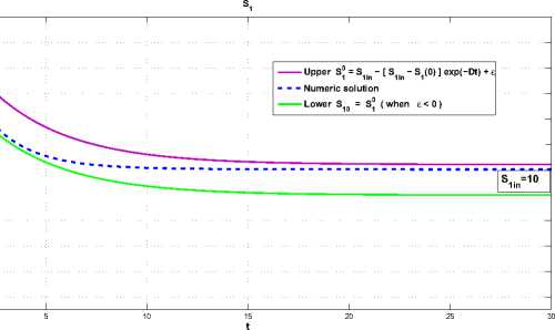
Fig. 1. Tending of a graph to S _{1 in} a s t ^ x . The parameters for simulation from [2]

Fig. 1 shows that the solution tends to the value S _{1 in} a s t ^ x . In the process, this represents that bacteria feed on the substrate S ₁ over time.

M.M. Higuera, A.V. Sinitsyn

Table

The solution to S 0

Parameter	Value	Units	SD
S 1(0)	5	[g/1]
D	0,395	[d - 1	0,135
S 1 in	10	[g/1]	6,4

Now we look for a semi-trivial upper-solution X^ for equations (15b) and (24). From

Definition 5

X 1°

-

µ 1 max

^S 1⁰

S ° + K s 1

-

αD

X ° >  0 .

Taking (16) and (24) in (15b), with c8 = S 1 in — S 1(0) we obtain

X 1°

-

µ 1 max

S I in - c 8 exp( —Dt )

^S 1 in - ^c 8 ^exP⁽ -Dt ) + KS ₁

- αD

X 1° = 0

then

X ° = c 9 *

№ 1 max ^S 1 in

[ c 8 exp ( —Dt ) ( S 1 in + K s 1 — c 8 exp( — ID t ))] ^{D ( S 1} in ⁺ KS i) ^{[ S} 1 in + KS 1 ^{— c} 8 ^{exp( —}Dt ^{)] D}

* exp ( —a D t )

and a graphic representation is Fig. 2 shows that the upper solution X ° presents condition washout.

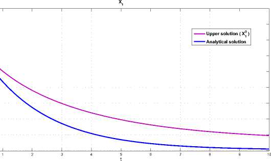
Fig. 2. The graph of the solution X ₁ tending to 0 a s t ^ to. The parameter values are taken from Table, with initial condition X ₁(0) = 0 , 5

Conclusions

In this paper we presented a study of existence of lower and upper solutions of a system of ordinary differential equations modelling acidogenic stage process of AD. Inverse order of lower and upper solutions with respect to variables was considered. We are well aware that this is only the first step in the complete study of the problem. The next step is to consider the V.M. Matrosov comparison principle to explore the global stability of solutions and a complete study of bifurcation (here readers may refer to monographs [8, 9]).

The first author is partially supported by SNI-CONACYT and thanks the University of Ibague in Colombia for their support and also thanks to the doctoral program in mathematics at the Faculty of Mathematics at the University of Veracruz in Mexico.