External boundaries of pole localization region formulation for transfer function with interval-given parameters

Introduction. In classical automatic control theory, parameters of technological objects models and control systems are expressed in real fixed values, but in practice the exact parameter values and coefficients are unknown and can be represented as some tolerance interval values of a given parameter.

Referring to a number of works devoted to the study of systems with interval-given parameters [1–9], it can be noted that the boundaries of the pole localization region of the transfer function (TF) of these systems are obtained by calculating the roots of the characteristic equation at some discrete step of varied parameter changing, i.e. numerical construction of boundaries takes place. This approach allows to determine numerical values of root quality indicators for a given class of systems with some given accuracy and similarly to evaluate the stability of the system as a whole. However, it requires a lot of iterative calculations. In turn, when solving the problems of the regulator parametric synthesis, the absence of analytical dependence does not provide accurate understanding of how the changing values of parameters affect the quality indicators.

The above problems of synthesis and system analysis with interval-given parameters require analytical description.

Task Setting. The task for the third-order TF with interval-given parameters to obtain the analytical function describing the external region of pole localization at any parameter values within the specified intervals.

Obtaining basic dependencies. Let us assume that given is some 3rd order TF system with characteristic polynomial of

A ( s ) = a 3 s ³ + a 2 s ² + a_i s + a 0 .             (1)

Edges of root locus are formed by motion of polynomial roots (1) under changing value of one or several polynomial coefficients.

It is known that the roots of the cubic equation can be analytically found applying Cardano’s formula. Cardano's formula gives solution to the following cubic equation y3 + py + q = 0.                 (2)

To bring the original characteristic equation of the system (1) to the appearance (2), we obtain a set of coefficients of the equation

. a j -i — b n — j + 1 = —, j = 1, n , a_n

where n - order of the system characteristic polynomial (1). Values p and q will respectively equal

b ²

P — 3 + b2,

2 b ³ bb

q = —1---2 + b.

We will then substitute the obtained values p and q

into Cardano’s formula

q

y=3-- +

V 2

' q- + p- + 3!

q

qp

..

With regard to substitution s = y - a²- [10] 3 a ₃

s i,2,3 ⁽ a 3 , a 2 , ^a i , a 0 ) =

a

( u ( a 3 , a 2 , a i , a 0 ) + v ( a 3 , a 2 , a i , a 0 ) ) - -^, 3 a ₃

( u ( a 3 , a 2 , a i , a o ) e 2 + v ( a 3 , a 2 , a i , a 0 ) e i ) - a²- , 3 a ₃

( U ⁽ a 3 , a 2 , a i , a o ) e i + ^{v (} a 3 , a 2 , a i , a o ) e 2 ) ^- a²-, 3 a ₃

where

u ( a 3 , a 2 , a i , a o ) =

( 9 a ₃ a ₂ a_i — 27 a 0 a ₃ ²

2 a 23 +

A

— 9 a 3 a 2 a i + 2 a 2 ) + 4 ( 3 a i — a 2 )

54 a ₃ ³

.

v ( a 3 , a 2 , a i , a o ) =

Г 9 a ₃ a ₂ a _i - 27 a 0 a ₃ ²

2 a ₂ ³

A

,² - 9 a ₃ a ₂ a _i + 2 a ₂ ³ ) + 4 ( 3 a _i - a ₂ ² )

54 a

,

к

e2 = —

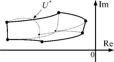
Fig. 1 Interval Root Locus with internal and external edges intersection

Рис. 1. Корневой годограф системы с наличием взаимного пересечения внешнего и внутреннего ребер

Using the property e^ — e2 и e22 — e1, the expression for the roots of the equation can be rewritten as s (a 3, a 2, a^, a о) —

a

u(a3,a2,a1,a0)e1 + v(a3,a2,a1,a0)e2 )

3 a ₃

k — {0,1,2}.(7)

In addition, the pole configuration will be determined by the discriminant equation value (2), the expression for which is

Q — q- + P- .

Let us consider the case of Q e ( 0; + « ) , which correlates with the pair of complex-conjugate poles and one real pole.

For a system with interval-given parameters, the edge of a multi-parameter root locus (MPRL) is formed by changing the value of one of interval parameters at fixed boundary values of other parameters. Thus, the analytical expression E^k_f^l for the MPRL edge when changing parameter values a_l can be determined according to (3) as

E kl = S k ( a i ), k = 1, n , l = 1, m (8) where n – order of characteristic polynomial, m – number of interval parameters.

Given that the presented expressions are obtained with respect to the coefficients at the degrees of characteristic equation, it is also fair to use dependency data for more complex types of uncertainties. For affine, polylinear, and polynomial uncertainties, coefficients at degrees in general form can be represented as a_k — ф ( q 1 , q 2 ,.., q l ) [11] and are further substituted into (8), having the following appearance

E k — S k ( ф ( q i ) ) , k — 1, n , l — 1, m .

Description of system pole boundary regions localization under the interval type of uncertainty. So-called external vertices must be selected to form the ex- ternal boundary of the TF system pole localization region with the parametric uncertainty of the interval type. The procedure for determining the membership of an MPRL vertex in a set of external vertices is based on the values of the departure angles. The angle of the edge departs from the vertex is defined as

0 — 180 °- E © k + E © i ,          (9)

Under parameter increase, or

under decrease [12-13], where © _k and © l - angles between real axis and vectors, directed from the pole under study to neighbor poles and zeros respectfully. The vertex will be referred to as external vertex in case all of its exit angles lie within the sector in 180⁰ [14].

It should be noted that when considering TF systems with interval-given parameters of the third order and higher, edge intersection connecting two external vertices and the edge connecting one external vertex with an internal vertex are possible, as shown in fig. 1.

Edges intersection is possible in case they come out of the same vertex and are formed by changing the values of the coefficients at degrees i , j for which the condition

|i - jj > 3 is met. For the coefficients under study with indexes i, j the following equation system can be formulated sin ((j - i )ф) — 0;

E ^azV\^{J +} z sin ( ( z ^- j ) ф )^— 0;

z

where i, j – the indices of vertex polynomial parameters which variation forms intersecting edges, z are the set of indices of the remaining coefficients of the vertex polynomial. Considering the part of the MPRL formed only by poles with a positive imaginary part, the angle ф will be defined by the expression ф —n-—,\i- j\ — 3,4,5... (12) Ii- j\

Substituting ф into the second expression (11), we obtain s . Knowing the module and argument, we will find the actual value of the edges intersection point U* . However, to correctly create the system of analytical expressions defining the boundary of localization region of a given system, we must define parametric coordinates of the point U* , i. e. interval parameter values ai,aj, under which the edges, coming out from the boundary vertex, created by the movement of these parameters possess a common point [15].

Numerical parameter values ai*,aj*in point U* may be obtained from equations s 2( ai, a 2, av a 0) = U *;

_ ⁵ 2 ⁽ a 3 , a 2 , ^a 1 , a j ) = U * ;

where ai,aj – changeable parameters , a2,a3 – fixed border values of corresponding parameters.

Example. Let us consider the system described by the 3-order TF with interval-given parameters and characteristic polynomial of

A(s) = [ a3 ] s3 + [ a2 ] s2 + [ a1 ] s + [ a0 ], where a3 = [0.7; 0.9],   a2 = [1.7; 2.2], a1 = [5.2;7.6], a 0 = [2.5;3.7].

Let us numerically build MPRL for a given system (fig. 2). Since MPRL is symmetrical to the real axis, only the part with a positive imaginary part is considered. Applying (9) and (10), we will define a set of external vertexes of the given system root locus. The obtained set of external vertexes makes the route: 5 ^ 7 ^ 3 ^ 4 ^ 12 ^ 10 ^ 14 ^ 13 ^ 5, with external boundary of transition 13 ^ 5 created by the part of the transition 13 ^ 5 and 5 ^ 6. For this system the edge 5 ^ 6 is formed via polynomial root P5^6(s) = a3s3 + a2s2 + a1 s + [a0 ], with the edge 13 ^ 5 root transition /3 >s(s) = [a3]s3 + a2s2 + a1 s + a0. Indexes of the given edges coefficients differ by 3, which is a must requirement for intersection. Therefore, the index of variable parameter of one edge is i = 3 , of the other is j = 0 . Substituting the obtained values into (11) and (12), 2n we obtain ф = —, |s| = 2.3636. Applying Eulers formula, we will receive the point of intersection U* =-1.1818 + 2.047i. Solving (13), we obtain a3* = 0.7415 and a0* = 3.047.

Having obtained a set of external vertices, a set of variable parameters forming the edges connecting the external vertices, and having determined the presence and further coordinates of the specific point of edges intersection, we can form a system of analytical expressions defining the borders of the pole system location region (fig. 3)

	f 1 ( a 1 ) = u ( a 3 , a 2 , a b a 0 ) e 2 k	+ v ( a 3 , a 2 , ab a 0 ) e 1 k	a - , a 1 el 3 a 3		a<; a 1 ] ;
	f 2 ( a 2 ) = u ( a 3 , a 2 , a 1 , a ^ ) e 2 k	+ v ( a 3, a 2, a 1, a 0) e 1 k	a , a2 3 a 3 2	€	a 2 ; a 2 J ;
	k f i ( a 0 ) = u ( a 3 , a 2 , a 1 , a 0 ) e 2 k	+ v ( a 3, a 2, a 1, a 0) e 1 k	a 2 - т—, a 0 3 a 3	€	_ a 0 ; a 0 J ;
	f 1 ( a 3 ) = u ( a 3 , a 2 , a 1 , a 0 ) e 2 k	+ v ( a 3, a 2, a 1, a 0) e 1 k	a 2 - ^, a 3 3 a 3	€	_ a 3 ; a 3 ] ;
F ( a 3 , a 2 , a 1 , a 0 ) = <	k f ; ( a 1 ) = u ( a 3 , a 2 , a 1 , a 0 ) e 2 k	+ v ( a 3, a 2, a 1, a 0) e 1 k	a 2 - 7=, a 1 3 a 3	€	a 1 ; a 1 J ;	(14)
	f 6 ( a 2 ) = u ( a 3 , a 2 , a; a " ) e 2 k	+ v ( a 3, a 2, a 1, a 0) e 1 k	a -—, a 2 3 a 3	€	a 2 ; a 2 J ;
	f 7 ( a 0 ) = u ( a 3 , a 2 , a , , a „ ) e 2 k	+ v ( a 3, a 2, a 1, a 0) e 1 k	a - ^,a 0 3 a 3	€	_ a 0 ; a 0 ] ;
	f , ( a 3 ) = u ( a 3 , a 2 , a ^ ^) e 2	+ v ( a 3, a 2, a 1, a 0) e 1 k	a -:;—, a 3 3 a 3	€	a 3* ; a 3 J ;
	f , ( a 0) = u ( a 3 , a 2 , a . , a 0 ) e 2 k	+ v ( a 3, a 2, a 1, a 0) e 1 k	a - ^T, a 0 3 a 3	€	a 0* ; a 0 J .

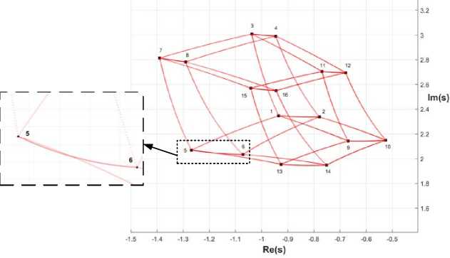
Fig. 2 Interval Root Locus for the given system

Рис. 2. Корневой годограф заданной системы

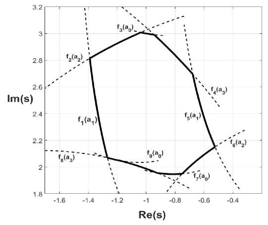
Fig. 3. Piecewise function F ( a ₃, a ₂, a ₁, a ₀) forming the external boundary of poles localization region

Рис. 3. Кусочно-заданная функция F ( a ₃, a ₂, a ₁, a ₀) , образующая внешнюю границу области локализации полюсов ПФ системы

Conclusion. The work justified a need for analytical approach to the study of systems with interval-given parameters. The analytical approach allows to obtain a clear idea of the system behavior, as well as formalize the synthesis procedure. According to the results of the study, analytical expressions for edges were worked out, a piecewise function for the boundary of the pole localization region of the 3-order transfer function with intervalgiven parameters was obtained. Furthermore, a numerical example was considered, the results of which confirm the above-mentioned theoretical research.